Things covered here:

• Some comments on assembling individual samples vs co-assembling multiple samples together
• Assembling a metagenome
• Visually identifing clusters of contigs (“binning”) based on sequence composition and coverage

Intro

There are lots of awesome things you can do with metagenomics. Here’s an overview that tries to highlight some common approaches:

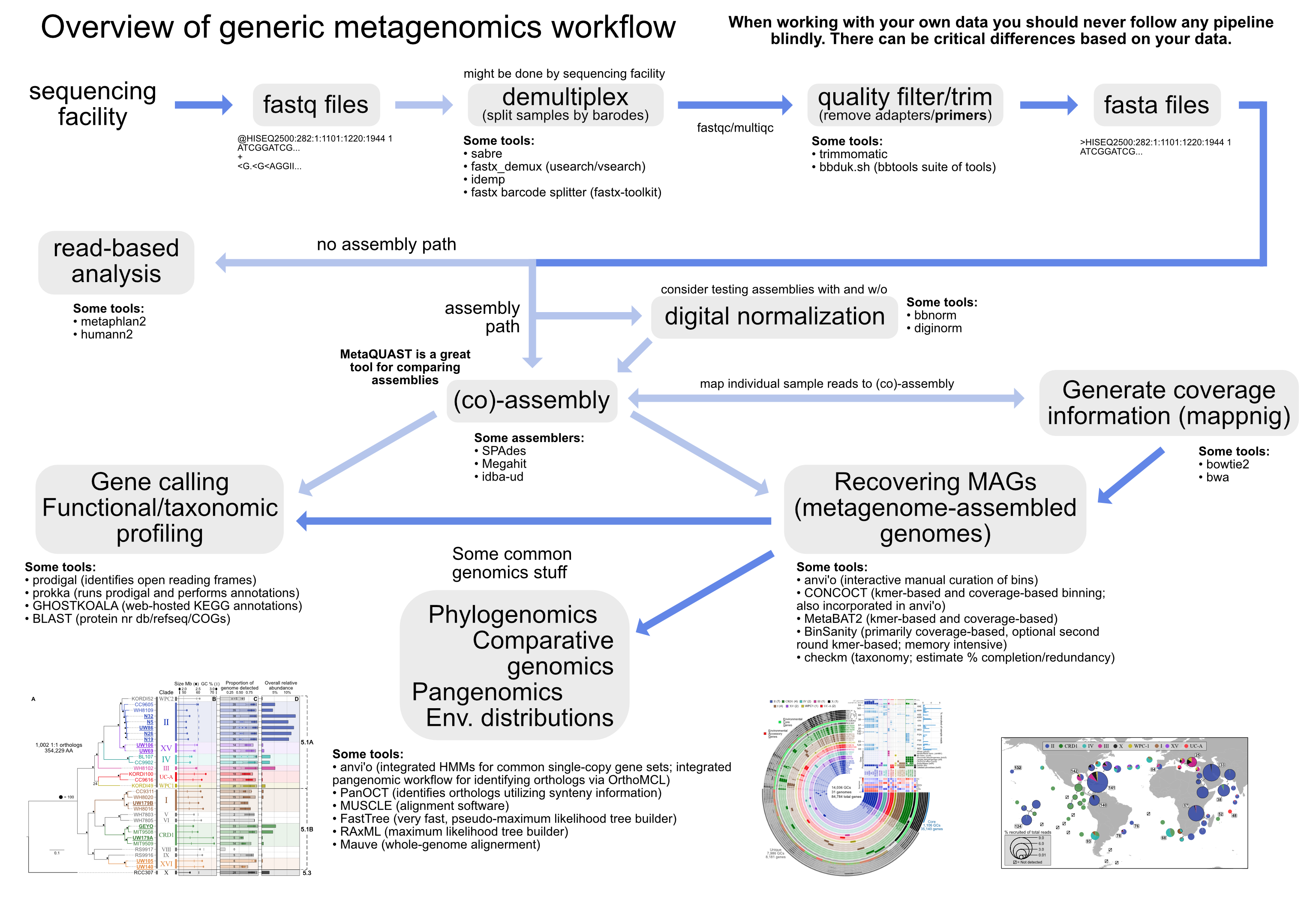
Recovering genomes from metagenomes has become a powerful tool for microbial ecologists. Here we will assemble a metagenome, and go through the process of “binning” our assembled contigs into groups based on coverage and sequence composition using the analysis and visualization platform anvi’o.

NOTE: Even the highest quality genomes recovered from metagenomes are not the same as isolate genomes. It depends on the data and assembly, but in general they are more of an agglomeration of very closely related organisms from the sample due to the assembly process and fine-scale variation that exists in microbial populations. They are being more frequently referred to as “metagenome-assembled genomes”, or MAGs, to better convey this.

Software needed

We will be using several different tools here, all are installable with conda. This line should do the trick:

conda install -y bowtie2 anvio diamond

Our practice data

To work with a smaller dataset here that will let us do things in a reasonable amount of time, we’re going to be working with a relatively simple microbial community here that comes from metagenomic sequencing of an enrichment culture of the nitrogen-fixing cyanobacterium Trichodesmium. Metagenomics still takes a lot of time, so we’re going to start with data already quality trimmed/filtered here, though assessing the quality and trimming/filtering as needed as laid out in this lesson should pretty much always be the first step. To lighten the processing load the majority of Trichodesmium (target cultivar) reads have also been removed. Despite this, there are still some steps that would take a bit too long to just wait for, so in those cases there will be examples of how the code would be run, but we’ll just pull result files from a subdirectory that comes with the data download so skip some of the more time-consuming steps 🙂

Downloading the practice data should only take about 3 or 4 minutes (it’s ~1.5 GB):

cd
curl -L https://ndownloader.figshare.com/files/12389045 -o metagen_tut.tar.gz
tar -xzvf metagen_tut.tar.gz
rm metagen_tut.tar.gz
cd metagen_tut

This main directory we just changed into holds 3 subdirectories: “data”, which holds our 4 samples’ forward (R1) and reverse (R2) reads (though they are empty here to save storage space and transfer time); “results”, which holds our result files we’ll use from time to time to skip longer steps; and “working”, where we are going to be running our commands from. So let’s take a look at it with ls, and then change into the “working” directory (which should be empty right now):

ls
cd working/
ls

I typically make a “samples.txt” file that contains each of my sample names when I start with a new project. This is because I’ll often use it for some loops as we’ll see below. One way to do that would be like this (with a complete breakdown to follow):

ls ../data/*.gz | cut -f3 -d "/" | cut -d "_" -f1,2 | uniq > samples.txt

Code breakdown: build this code up one command at a time (press enter for each part, then add the | and the next part)

• ls is the starting command, and we’re telling it to list all the files that end in “.gz” from our “data” directory, then we pipe | the output from that into the next command
• cut pulls out specific columns. It uses tabs as default to be the character that separates columns, but we are adding a flag to modify that
  • -d is how you specify the delimiter (what separates columns) for cut, here we are saying to use the underscore character _, just because that would allow us to split the file names up where we wanted (working to get just the sample names with no extensions or read direction info)
  • -f stands for “field” (column), and this is where we tell cut that we want the first and second column (which based on our delimiter grabs “Sample_A” for example). Right now we’d have double lines for each sample, which isn’t what we want in our file of sample names, so we’re going to pipe | this output also into one last command
• uniq removes duplicate lines and leaves only singles of each (note things need to be sorted for uniq to work, here that was already done, but you should look into it further in the future if unfamiliar with it)
• > finally we redirect the final output to a file names “samples.txt”. Check out the contents with cat samples.txt.

And now we’re ready to get to work!

What is a co-assembly?

“Co-assembly” refers to performing an assembly where the input files would be reads from multiple samples. This is in contrast to doing an independent assembly for each sample, where the input for each would be just the reads from that individual sample. Three major benefits of co-assembly include: 1) higher read depth (this can allow you to have a more robust assembly that captures more of the diversity in your system, but not always); 2) it facilitates the comparison across samples by giving you one reference assembly to use for all; and 3) it can substantially improve your ability to recover genomes from metagenomes due to the awesome power of differential coverage (you can download a slide showing how coverage is used to do this from here -> keynote, powerpoint).

To co-assemble or not to co-assemble?

Though a co-assembly has its benefits, it will not be ideal in all circumstances. And as with most things in bioinformatics, there are no golden rules as for when it would be better to co-assemble multiple samples together over when it would be better to run individual assemblies on each. It could depend on many factors (e.g. variation between the samples, diversity of the communities, the assembler(s) you’re trying, you’re overall questions, who knows how many others things?, etc.), and there can be datasets where a co-assembly would give you a poorer output assembly than an individual assembly would. So it is something you should consider with each dataset you work with, and if you are unsure and have the time/resources, then trying and assessing the outcome is always good practice.

Co-assembly

Above, we briefly touched on some plusses and minuses of co-assembly vs individual-sample assembly. Here we are working with 4 samples from an enrichment culture, and the communities should be pretty well constrained - certainly relative to complex environmental samples like, say, a transect across soil. That would be harder to decide, but for us, it’s a pretty safe start to go with a co-assembly.

There are many assemblers out there, and the reason each has a paper showing how it beats others is because every dataset is different. Some assemblers work better for some datasets, and others work better for others. That’s not to say all are magically equally good in every sense, but most that gather a following will out-perform all others under certain conditions. I typically try several (some well-known assemblers include SPAdes, Megahit, idba-ud, Minia), and compare them with QUAST (for individual genome assembly) or MetaQUAST (for metagenome assemblies). Choosing the “best” assembly is not straightforward and it can depend on what you’re doing, there is some more on that here if you’re interested, along with an example of testing assemblies/options and comparing them.

In this case, here is how the command would be run with the Megahit assembler. But even with the smaller dataset we’re using, this takes about 40+ minutes on our cloud instances using 4 cpus. So rather than running this, we’re just going to look at the command and then pull the assembly output file from our results directory.

  ## don't run this, would take about 40+ minutes ##
# megahit -1 ../data/Sample_A_1.fastq.gz,../data/Sample_B_1.fastq.gz,../data/Sample_C_1.fastq.gz,../data/Sample_D_1.fastq.gz \
# -2 ../data/Sample_A_2.fastq.gz,../data/Sample_B_2.fastq.gz,../data/Sample_C_2.fastq.gz,../data/Sample_D_2.fastq.gz \
# -o megahit_default -t 4

Code breakdown:

• megahit is the command, it is specifying the program we are using
  • -1 is for specifying the forward reads. Since we are doing a co-assembly of multiple samples, we could have stuck them altogether first into one file, but megahit allows multiple samples to be added at once. Notice here we are specifying all the forward reads in a list, each separated by a comma, with no spaces. This is because spaces are important to the command-line’s interpretation, whereas commas don’t interfere with how it is interpreting the command and the information gets to megahit successfully.
  • -2 contains all the reverse read files, separated by commas, in the same order.
  • -o specifies the output directory (the program will produce information in addition to the final output assembly)
  • -t specifies that we want to use 4 cpus (some programs can be run in parallel, which means splitting the work up and running portions of it simultaneously)

After waiting for that to finish, we would have the “megahit_default” directory that is currently within our “results” directory. So we’re just going to copy over that final output fasta file (our co-assembly) into our working directory:

cp ../results/megahit_default/final.contigs.fa .

If you glance at this file, with head final.contigs.fa for example, you can see there are spaces and some other special characters in the headers (the lines that start with “>”). This can be problematic for some tools, and it’s better to have simplified headers if you can. There are lots of ways to make modifications like that, and some scripts already exist. Anvi’o happens to have one, so we’re just going to use that here. We’re also going to filter out any contigs that are shorter than 1,000 bps. Whether you’d want to do this normally or not is up to the researcher, but that is roughly the average size of a bacterial gene, and the smaller contigs become the more difficult it becomes to get useful information out of them.

anvi-script-reformat-fasta final.contigs.fa -o contigs.fa -l 1000 --simplify-names

Code breakdown:

• anvi-script-reformat-fasta is the command, it is specifying the program we are using
  • the first “positional” argument (no flag needed) is specifying the input file (our assembly)
  • -o specifies the name of the output file
  • -l specifies we wanted to filter out sequences with fewer than 1000 bps
  • --simplify-names tells the program we want it to give all sequences a “clean” header (no special characters)

Mapping our reads to the assembly they built

Among other things (like enabling variant detection), mapping our reads for each sample to the co-assembly they built gives us “coverage” information for each contig in each sample, which as discussed above will help us with our efforts to recover metagenome-assembled genomes (MAGs).

Here we are going to use bowtie2 to do our mapping, and first need to create an index of our co-assembly:

bowtie2-build contigs.fa assembly

And here is where we would map our individual samples’ reads to our co-assembly, but mapping and converting the file formats to what we need would take ~30 minutes to run on all samples, so we’ll look at the commands here and how they are run, but don’t actually run them. This could be done one sample at a time like this…

Mapping

  ## do not run, takes a bit ##
# bowtie2 -x assembly -q -1 ../data/Sample_A_1.fastq.gz \
# -2 ../data/Sample_A_2.fastq.gz --no-unal \
# -p 4 -S Sample_A.sam

Code breakdown:

• bowtie2 is the command, it is specifying the program we are using
  • -x is where we specify the “basename” of the index we just built, which is “assembly”, bowtie2 will find all the appropriate files using that basename
  • -1 specifies the forward reads of the sample we’re doing
  • -2 specifies the reverse reads
  • --no-unal tells the program we don’t want to record the reads that don’t align successfully (saves on storage space)
  • -p specifies how many cpus we want to use
  • -S specifies the name of the output “sam” file we want to create (Sequence Alignment Map)

Converting sam to bam (Binary Alignment Map, these are compressed and what is required for our next tool)

  ## do not run, takes a bit ##
# samtools view -b -o Sample_A-raw.bam Sample_A.sam

Code breakdown:

• samtools is the main program, it is specifying the program we are using
  • view is the subprogram of samtools that we are calling
  • -b tells the program we want the output to be in bam format
  • -o specifies the output file name
  • the last “positional” arugment (no flag needed) tells it the input file, which is our sam file for this sample

Sorting and indexing our bam files (also needed for our next tool)

  ## do not run, takes a bit ##
# samtools sort -o Sample_A.bam Sample_A-raw.bam
# samtools index Sample_A.bam

Code breakdown:

• samtools is the main program again for each
  • sort in the first command is the subprogram of samtools that we are calling
  • -o specifies the output file name
  • the last “positional” arugment (no flag needed) tells it the input file, which is our sam file for this sample
• index in the second command is the subprogram of samtools that we are calling
  • the only “positional” arugment (no flag needed) tells it the input file, the output file is the same name but with an additional extention added of “.bai” for Binary Alignment Index

But we made a “samples.txt” file so we could do all of the above steps with a loop where each iteration is acting on one of our samples, which would look like this (code breakdown below):

  ## do not run, takes a bit ##
# for sample in $(cat samples.txt)
# do
#   bowtie2 -x assembly -q -1 ../data/"$sample"_1.fastq.gz -2 ../data/"$sample"_2.fastq.gz --no-unal -p 4 -S "$sample".sam
#   samtools view -b -o "$sample"-raw.bam "$sample".sam
#   samtools sort -o "$sample".bam "$sample"-raw.bam
#   samtools index "$sample".bam
# done

Code breakdown: The special words of the loop are for, in, do, and done.

• for – here we are specifying the variable name we want to use (“sample” here), this could be anything
• in – here we are specifying what we are going to loop through, in this case it is every line of the “samples.txt” file
  • $(cat ...) – this is a special type of notation in shell. The operation within the parentheses here will be performed and the output of that replaces the whole thing. It would be the same as if we typed out each line in the file with a space in between them
• do – indicates we are about to state the command(s) we want to be performed on each item we are looping through
  • within this block between the special words do and done, each line is the same as the commands run individually above on a single sample. Only here, everytime we want to specify where the sample names would change is where we put “$sample”. The $ tells the command line to “interpret” the word “sample”, and since we made “sample” our variable name at the start of the loop (“for sample in …”), that will change each iteration to a different sample name and provide the correct input and output files for each command.
• done – tells the loop it is finished
  
  Don’t worry if loops are confusing at first! They take a litting getting used to, and this not a lesson on loops, just a quick explanation. All bits of exposure help over time 🙂

As mentioned above, running in real time on our cloud instances this would take about 30+ minutes to complete. So here we’re just going to pull the appropriate results files (the final bam files, “.bam”, and their corresponding indexes, “.bai”) into our current working directory:

cp ../results/*.bam* .

Anvi’o Time!

Anvi’o is a powerful analysis and visualization tool that provides extensive functionality for exploring all kinds of ‘omics datasets. Here we are going to use it to visualize our metagenome and coverage from each sample, to help us see how recovering “genomes” from metagenomes works.

A much more detailed anvi’o metagenomics tutorial can be found here which starts from where we are (having our assembly fasta file and our sample bam files), and in general there are many tutorials and blogs at the merenlab.org site with lots of useful information for those interested in bioinformatics.

Building up our contigs database

The heart of Anvi’o when used for metagenomics is what’s known as the “contigs database”. This holds the contigs from our co-assembly and information about them. What information, you ask? All kinds! And lots of it will be generated over the next few steps.

Generate an anvi’o contigs database from our co-assembly fasta file (this first one can take about 15+ minutes, so we will look at the command but skip it and grab the output from the results directory):

  ## do not run, takes a bit ##
# anvi-gen-contigs-database -f contigs.fa -o contigs.db -n "my metagenome"

Code breakdown:

• anvi-gen-contigs-database is the main program we’re using. All anvi’o programs start with “anvi-“, so if you type anvi- and press tab twice, you can see a list of all that are available (and most, if not all, have a help menu if you enter the command followed by --help).
  • -f this is specifying the input fasta file (our co-assembly)
  • -o is specifying the name of the output database that is generated (it should end with the “.db” extension)
  • -n specifies a name for your project

This step at the start is doing a few things: 1) calculating tetranucleotide frequencies for each contig (uses 4-mers by default but this can be changed); 2) identifies open-reading frames (“genes”) with prodigal; and 3) splits long contigs into segments of roughly 20,000 bps (though does not break genes apart) – this splitting of contigs helps with a few things like visualization and spotting anomalous coverage patters (we’ll see how anvi’o helps us visualize coverage below).

Since we skipped that to save time, let’s copy over the contigs database from our results directory:

cp ../results/contigs.db .

Now that we have our contigs.db that holds our sequences and some basic information about them, we can start adding more, like:

Using the program HMMER to scan for a commonly used set of bacterial single-copy genes (from Campbell et al. 2013). This will help us estimate genome completeness/redundancy in real-time as we work on binning our contigs below (this should only take ~3 minutes).

anvi-run-hmms -c contigs.db -I Campbell_et_al -T 4

Code breakdown:

• anvi-run-hmms is the main program we’re using
  • -c our input contigs database
  • -I specifying which HMM profile we want to use (you can see which are available by running anvi-run-hmms --help, and can also add your own if you’d like)
  • -T specifies that we’d like to split the work among 4 cpus

NOTE: See the bottom of page 7 of the HMMER manual here for a great explanation of what exactly a “hidden Markov model” is in the realm of sequence data.

Use NCBI COGs for functional annotation of the open-reading frames prodigal predicted. This can be done with either BLAST or DIAMOND – DIAMOND is like a less sensitive, but faster form of BLAST (default is DIAMOND). To run this however, we’re first going to have to setup our COG database for anvi’o. Together this will take about 5:

anvi-setup-ncbi-cogs -T 4 --just-do-it
anvi-run-ncbi-cogs -c contigs.db  -T 4

Code breakdown:

• anvi-setup-ncbi-cogs is the main program to set up the anvi’o COG database
  • -T specifies that we’d like to split the work among 4 cpus
  • --just-do-it tells anvi’o to proceed with the COG setup without asking for any confirmations from us along the way
• anvi-run-ncbi-cogs is the main program we’re using
  • -c our input contigs database

Assign taxonomy with a tool called Centrifuge to the open-reading frames prodigal predicted. This step takes having a database setup and takes some time to run. There are good instructions at the anvi’o tutorial for importing taxonomy, and here are the commands that were used to generate what’s in our results file:

  ## do not run, takes a bit and a database setup ##
# anvi-get-sequences-for-gene-calls -c contigs.db -o gene_calls.fa
# centrifuge -f -x /media/eclipse/centrifuge_db/nt/nt gene_calls.fa -S centrifuge_hits.tsv -p 20

Code breakdown:

• anvi-get-sequences-for-gene-calls is the main program we’re using
  • -c our input contigs database
  • -o specifies the output file name we want to write the sequences for our genes in fasta format
• centrifuge is the command used to assign taxonomy
  • -f tells the program the input file is in fasta format
  • -x points to where a pre-built “centrifuge” database is stored
  • the “gene_calls.fa” positional argument (no flag preceding it) is the input file
  • -S specifies the name of the main primary output file
  • -p specifies splitting the job across 20 cpus (this part was run on a different server, our clouds only have 6 cpus)

So we aren’t running that now, but let’s pull the results files we need into our working directory, and then import them into our contigs database:

cp ../results/*tsv .
anvi-import-taxonomy-for-genes -c contigs.db -i centrifuge_report.tsv centrifuge_hits.tsv -p centrifuge

Code breakdown:

• anvi-import-taxonomy-for-genes is the main program we’re using
  • -c our input contigs database
  • -i specifies the required centrifuge report file (was generated by the centrifuge command we skipped)
  • the positional argument “centrifuge_hits.tsv” specifies the primary centrifuge output file (was also generated by the centrifuge command we skipped)
  • -p specifies which type of input we are giving anvi’o. Since we can import taxonomy information to anvi’o provided from many different tools, how you get it into anvi’o can vary. In some cases tools are used frequently enough that anvi’o has built in to it a way to read the outputs. That is the case with centrifuge.

Profiling our samples

Ok, now that our contigs database has all kinds of information about our co-assembly contigs, we are now going to provide information about each of our samples to anvi’o so it can then integrate everything together for us. Each sample will have what’s known as a “profile database” that will keep information about that sample – like how many reads mapped to each contig and where. This step is surprisingly fast for all that it’s doing, but it would still take about 25+ minutes on our cloud instance. So we’re going to skip running these, but take a look at how it would be done.

We can do this for one sample like this:

  # do not run, takes a bit ##
# anvi-profile -i Sample_A.bam -c contigs.db -T 4

Code breakdown:

• anvi-profile is the main program we’re using
  • -i specifies the sample-specific input bam file
  • -c our input contigs database
  • -T specifies how many cpus to use

But just like above, we can do this with a loop (revisit the loop notes above for more explanation of what’s going on here)

  ## do not run, takes a bit ##
# for i in $(cat samples.txt)
# do 
#   anvi-profile -i "$i".bam -c contigs.db -T 4
# done

The last step is to merge all of these together into one anvi’o “profile”, so that we can consider them all together. This is done as follows:

  ## do not run ##
# anvi-merge */PROFILE.db -o merged_profile -c contigs.db

Code breakdown:

• anvi-merge is the main program we’re using
  • the first positional argument (no flag) specifies the sample-specific input profile databases. For each sample, when we ran anvi-profile above, the output created a subdirectory of results. By providing the * wildcard here followed by a /PROFILE.db we are providing all of them as inputs to this command.
  • -o the output directory
  • -c our contigs database

We skipped those steps to save some time, but lets copy over the results “merged_profile” directory now:

cp -r ../results/merged_profile/ . # the -r is required to copy the directory and its contents

Visualization

Ok! Now the payoff for all that hard work we just did. We are going to launch anvi-interactive which allows us to see our metagenome and how each sample’s reads recruited to it. This is why we had to sign in a little differently, to be able to host the website we are going to interact with so that we could get to it from our local computer.

anvi-interactive -p merged_profile/PROFILE.db -c contigs.db --server-only -P 8080

After running that on your cloud instance, go to your computer’s web browser and go to this address “http://localhost:8080” (Chrome is ideal for anvi’o, but if you don’t have that then whatever you’ve got will probably still be cool). Once that loads up, click the “Draw” button at the bottom left and you should see the metagenome appear 🙂

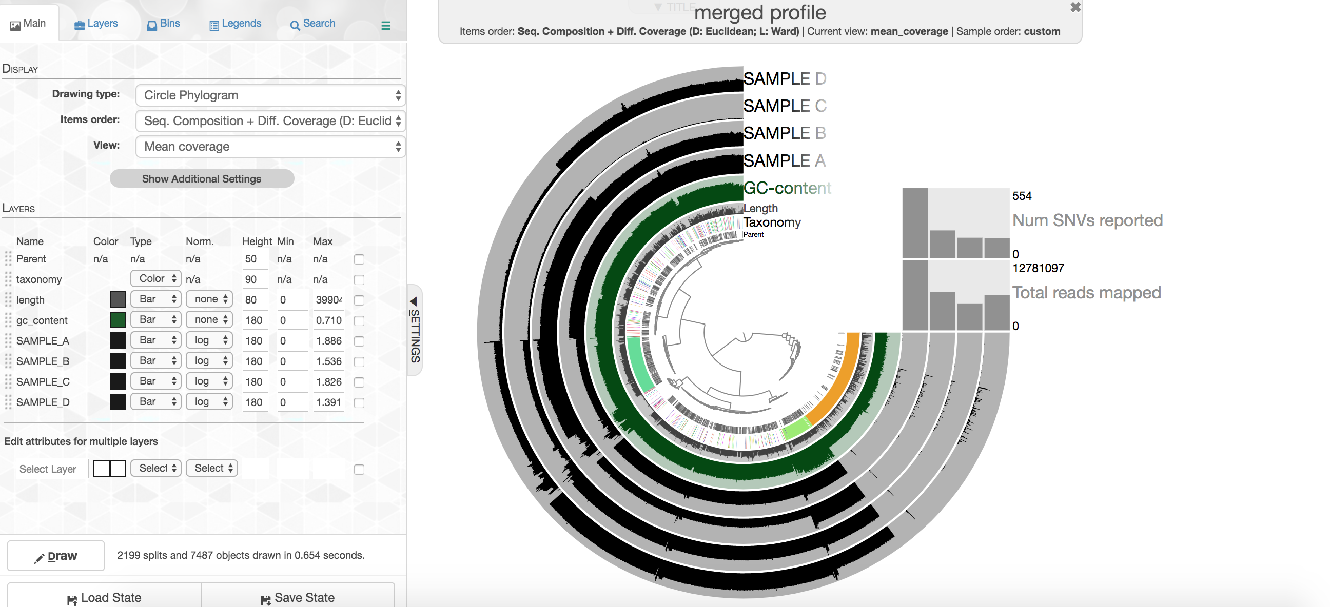
So there is a lot going on here at first glance, especially if you’re not yet familiar with how anvi’o organizes things. The interactive interface is extraordinarily expansive and I’d suggest reading about it here and here to start digging into it some more when you can, but here’s a quick crash course.

At the center of the figure is a hierarchical clustering of the contigs from our co-assembly (here clustered based on tetranucleotide frequency and coverage). So each tip (leaf) of the central clustering represents a contig (or a fragment of a contig as those longer than 20,000 bps are split into pieces of ~20,000 bps as mentioned above). Then radiating out from the center are layers of information (“Parent”, “Taxonomy”, “Length”, “GC”), with each layer displaying information for each corresponding contig (leaf/tip). Beyond those, we get to our samples. For each sample layer, the visualization is showing the read coverage for that sample to each contig as you travel around the circle.

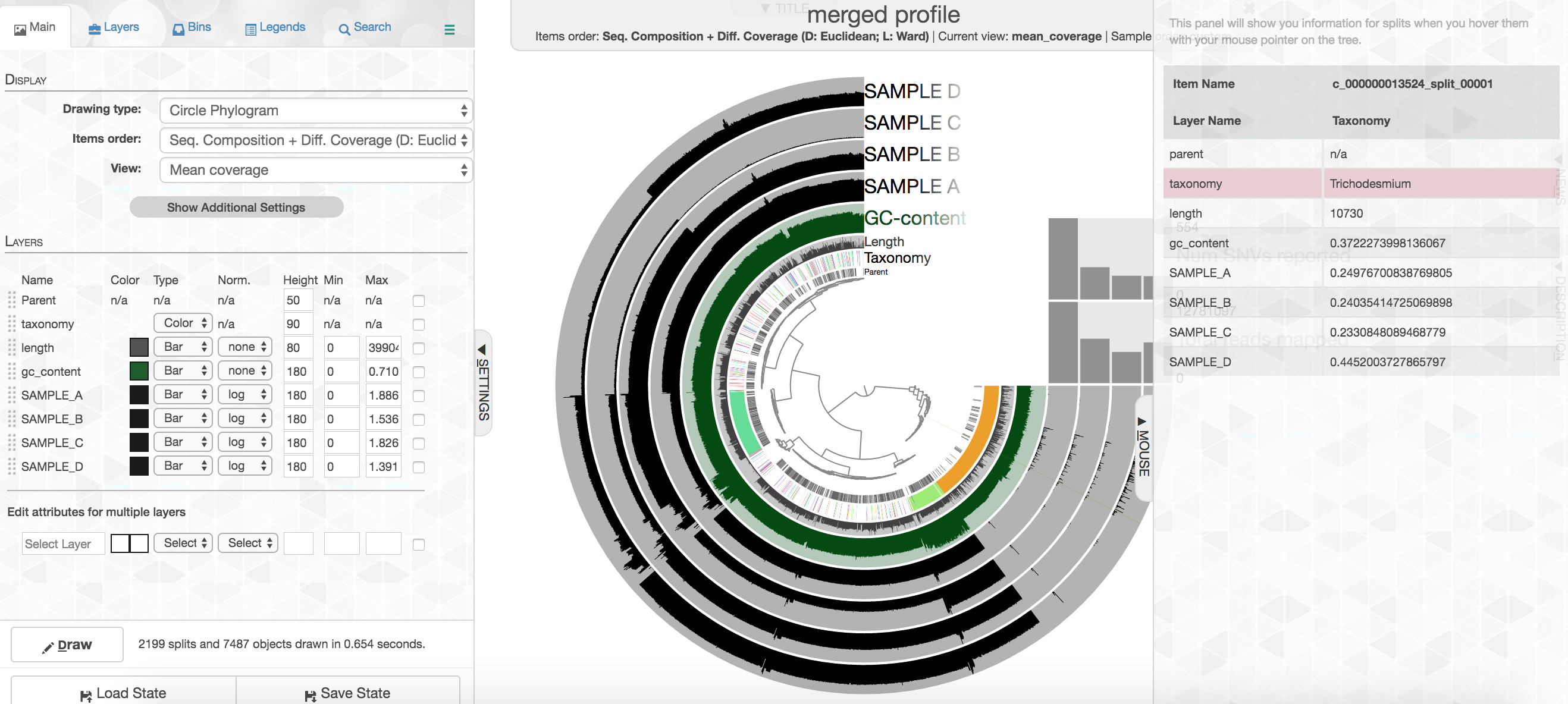
Let’s look at the taxonomy layer for a second, if you press the M key on your keyboard, a panel should pop out from the right side with information. Then if you hover over the taxonomy bar you will see the taxonomy called for genes on that particular contig. Here is an example:

Your colors will probably be different, but that doesn’t matter. Try to find the cluster of contigs that represents Trichodesmium. If you click on the “Bins” tab at the top left, and then select the branch on the tree at the center that holds all the Trichodesmium contigs, you will see a real-time estimate of % completion/redundancy.

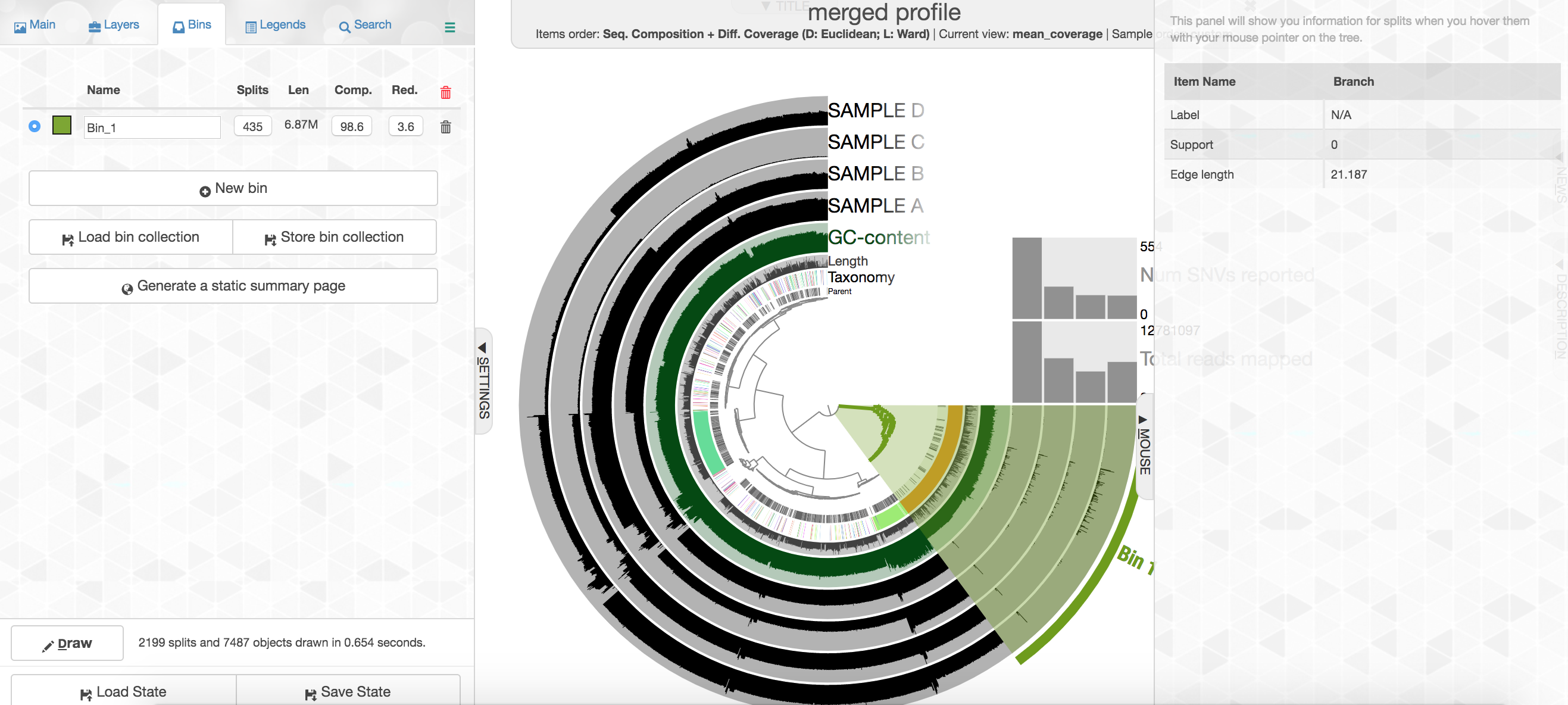
And we can see in the left pane that we selected 435 splits (contigs and/or split contigs due to length), with a total length of 6.87 Mbps, with an estimated 98.6% completion and 3.6% redundancy – remember estimated percent completion and redundancy comes from the bacterial single-copy genes we scanned for with anvi-run-hmms above. (This is pretty good, but Trichodesmium has a very strange genome for a prokaryote with a lot of long, repetitive regions that don’t assemble well, so we’re actually about 1 Mbps short of what would be expected.) As mentioned above, to shrink the dataset to make it more manageable most of the Trichodesmium reads have been removed, which is why the coverage patterns across the samples for Trichodesmium look strange, so don’t pay too much attention to that. Let’s move on.

In the panel to the left, click “New bin”, and let’s look at some of these other clusters of contigs. Try to find the Alteromonas cluster, and then select the branch that holds it.

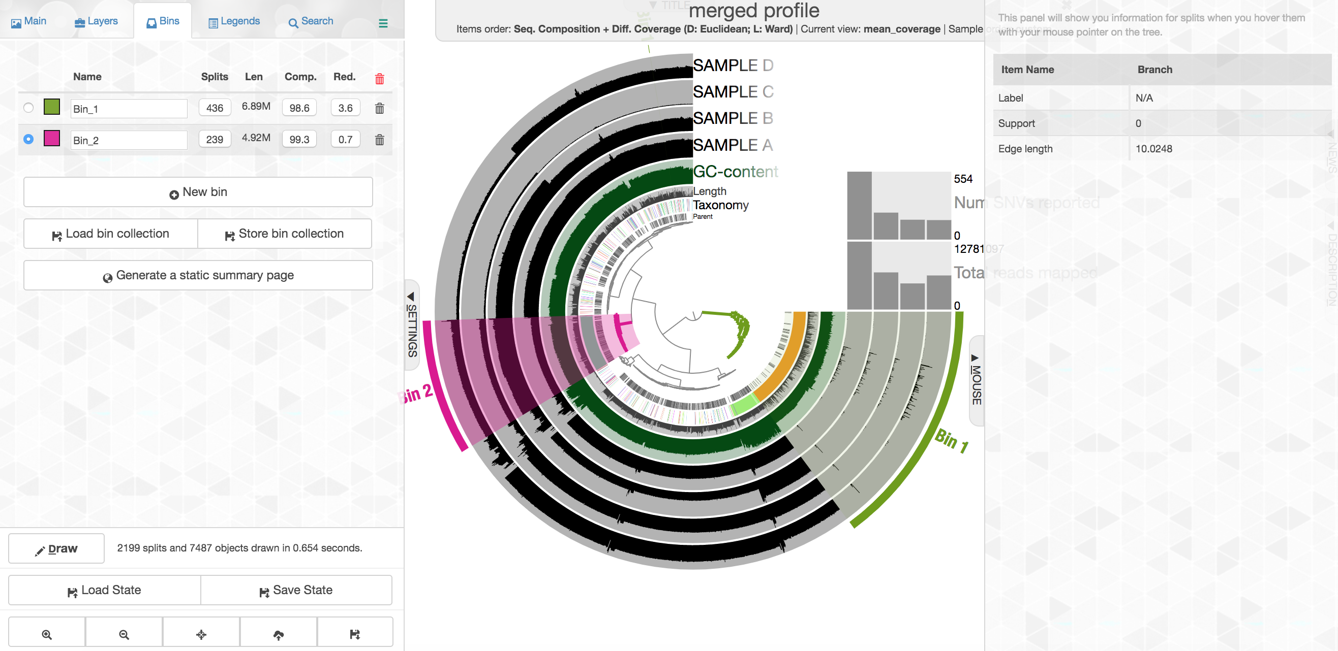
This ones says 4.92 Mbps which is pretty spot on for an Alteromonas, with an estimated 99.3% complete and 0.7% redundancy. Here we had the taxonomy clearly helping to define this group of contigs, but that’s very dependent on databases. Imagine we didn’t have the taxonomy guiding us, take a close look at the coverage of reads from the 4 different samples across these contigs:

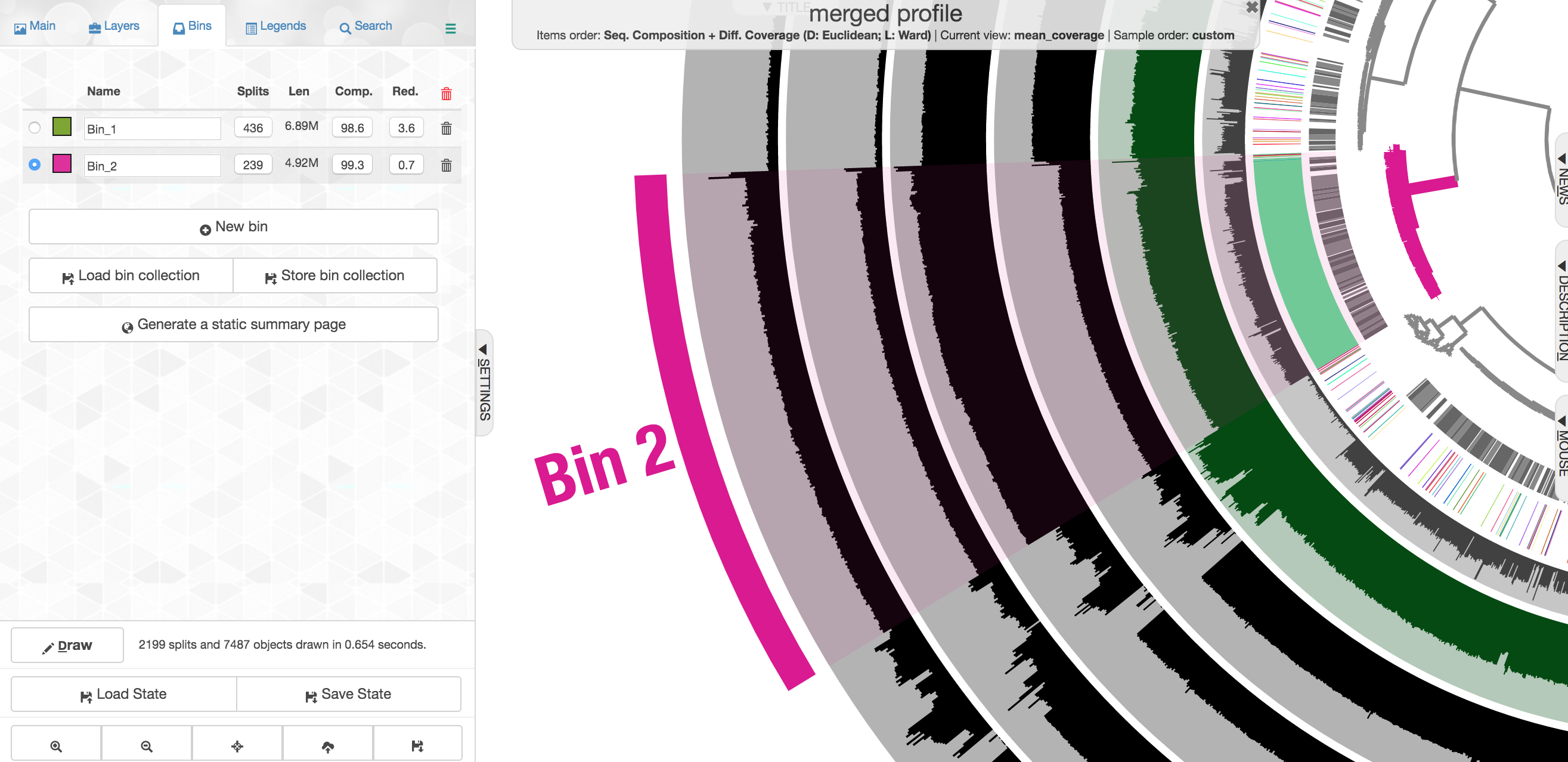
Note across the samples (the rows wrapping around the circle), the coverage of these contigs varies, but that within a sample it is pretty consistent across these selected contigs. Meaning, Sample B seems to have the highest coverage for these contigs, but evenly across, and Sample C seems to have the lowest, but again consistent within that sample. This is what we would expect the coverage to do if these contigs all came from a similar source, and that source as a whole was in a different abundance in different samples.

Let’s look at one where the taxonomy doesn’t help as much. First click “New bin” again at the left first, then select this cluster of contigs:

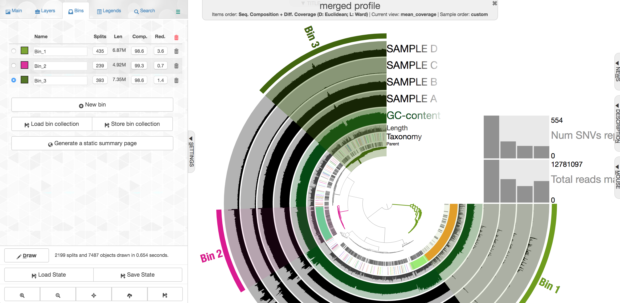
Note again how drastically the coverage shifts across samples, but how consistent it is within a sample. This is currently the most powerful tool we have for attempting to recover genomes from metagenomes. There are some contigs with pretty different coverage in the middle here, and they also have a pretty drastically different GC content:

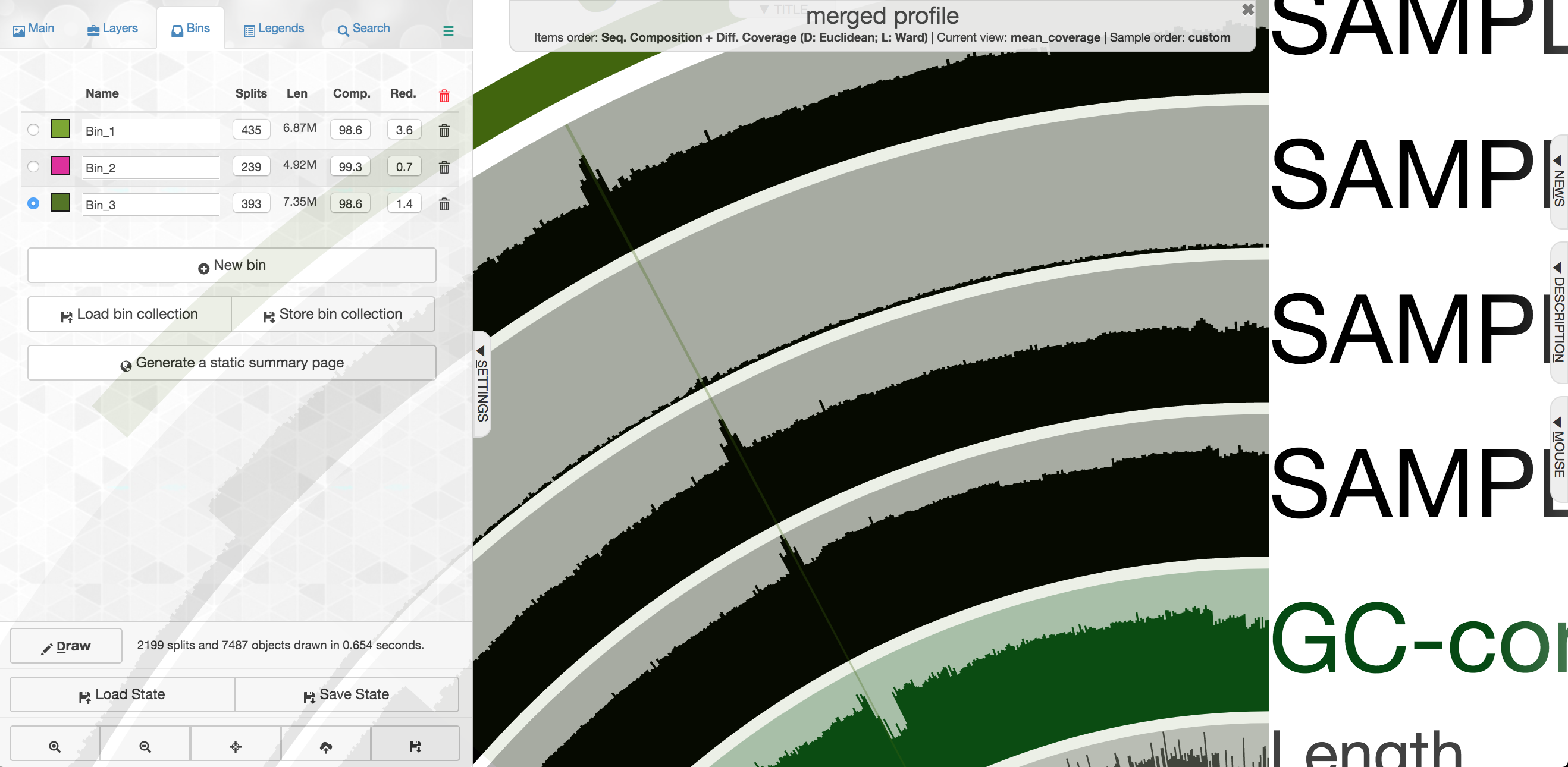
So let’s go one layer deeper and take a quick look at this. If you “right” click on one of the specific contigs, you’ll get a menu where you can select “Inspect”:

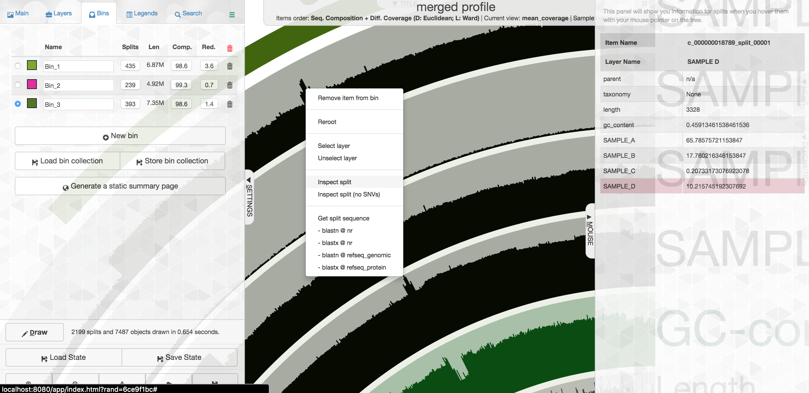
This will open that particular contig in a separate browser window. Here is opening contig “c_000000018789_split_00001”:

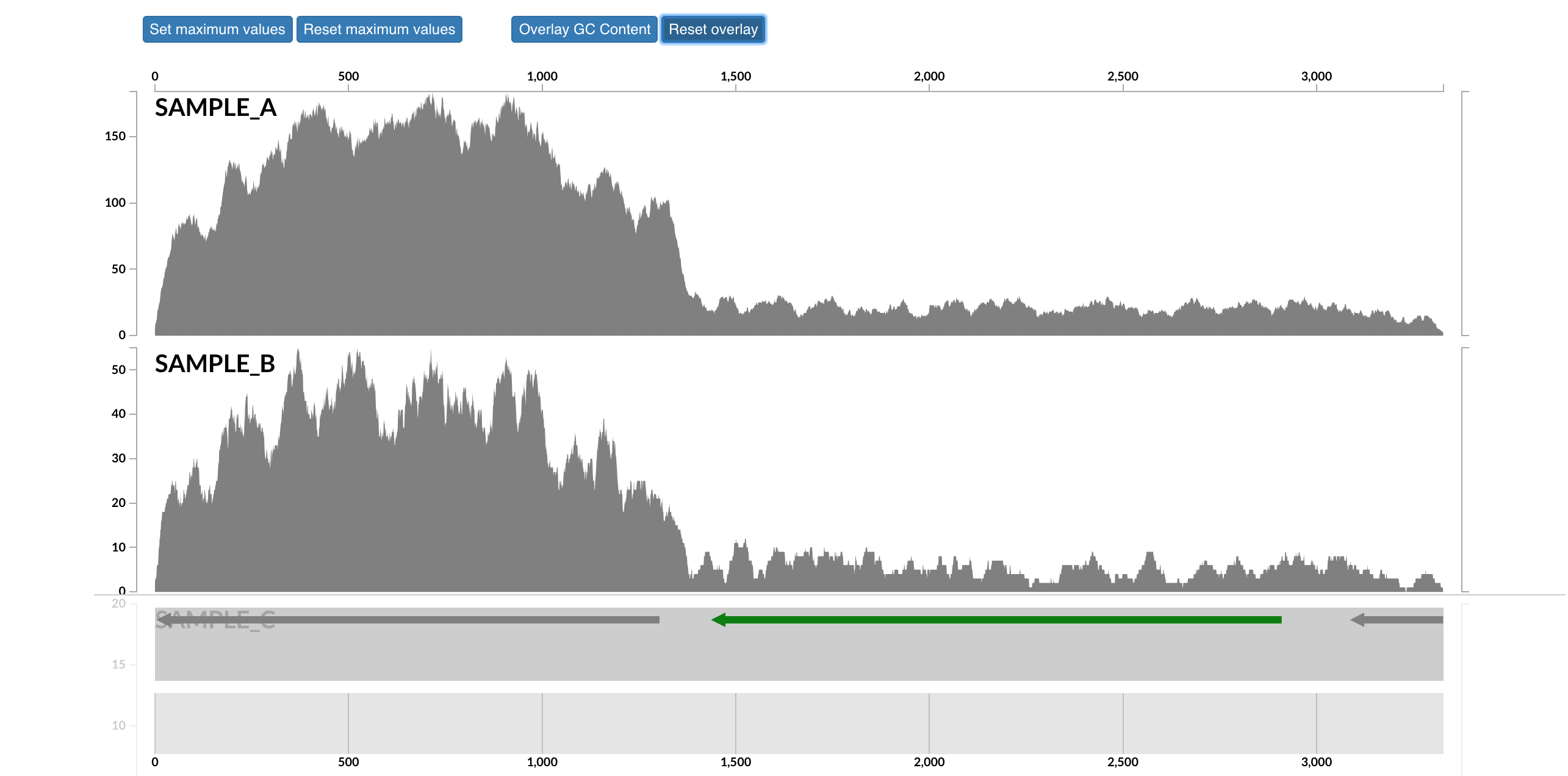
Here each row is a sample, the x-axis is the contig laid out, and the peaks show read coverage on that contig. If we look to the right we can see the drop in coverage. This overlaps with an annotated gene on the bottom (genes are arrows, annotated are green, not annotated are grey). If we click on that green arrow, we can see what the gene was annotated as:

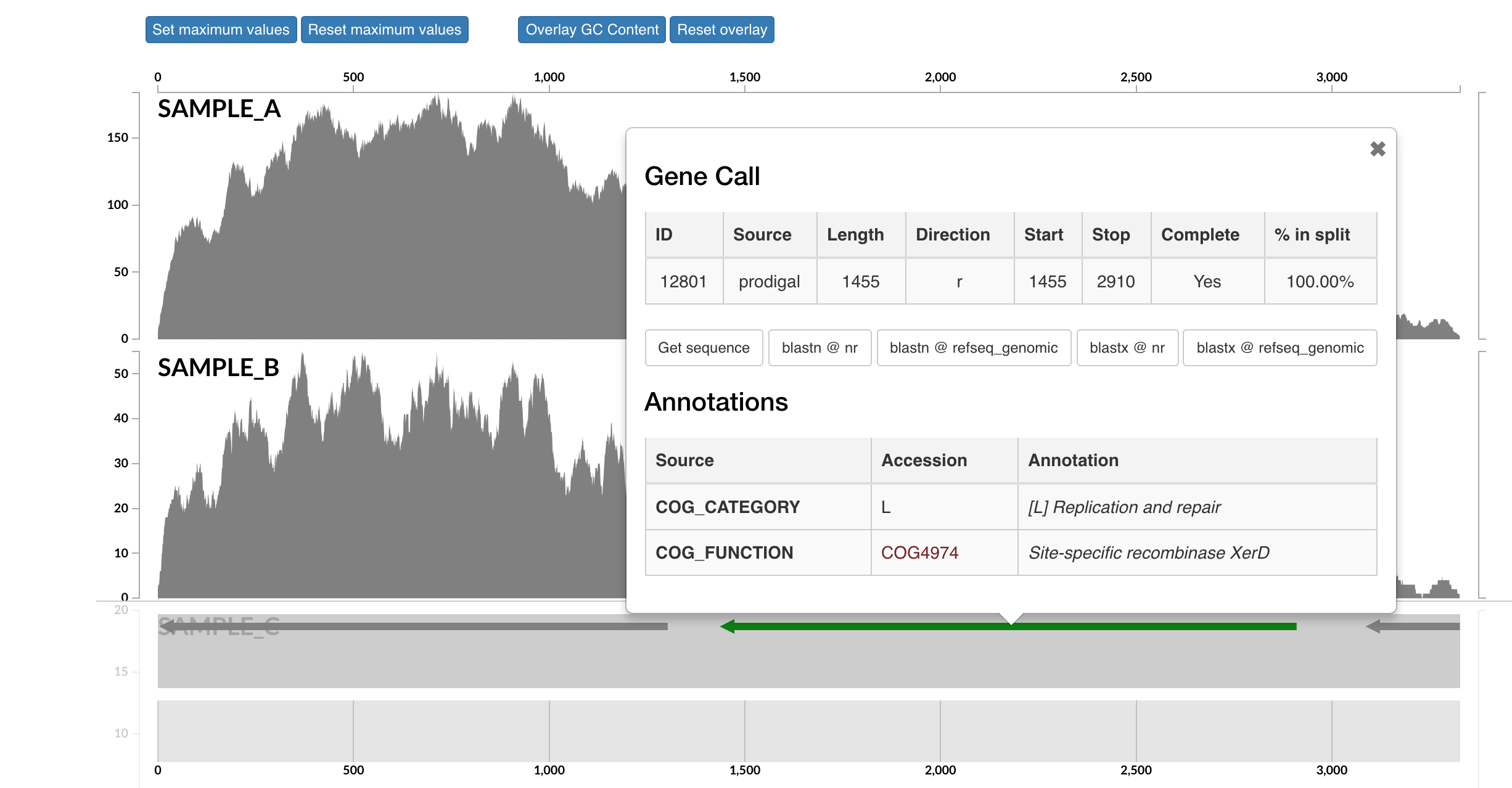
It seems the gene underlying the drop extreme drop in coverage across all samples was annotated as a site-specific recombinase. I don’t know much about these, but apparently they can be involved with recombination or DNA rearrangements. Maybe this was an artifact of assembly and shouldn’t be a part of our bin here. If you select “Get sequence” from the gene window, you can quickly go to NCBI and blast it if you’re curious. Running a BLASTX reveals the top hit as Phaeodactylibacter xiamenensis, which is what this bin actually comes from in this case (that’s known from further work not included here). But this sort of interface is where you could do meticulous manual curation of bins you were recovering by looking at things like coverage across samples.

Exporting our bins

Now that we’ve selected 3 bins, if we want to export them from anvi’o we need to save them first. To do that, on the “Bins” pane at the left of the main interactive screen, you would select “Store bin collection”, and give it a new name like “my_bins” and click OK. Then one way we can summarize them is by clicking “Generate a static summary page” in the “Bins” pane, and then select the new collection you made, and then click “Generate”:

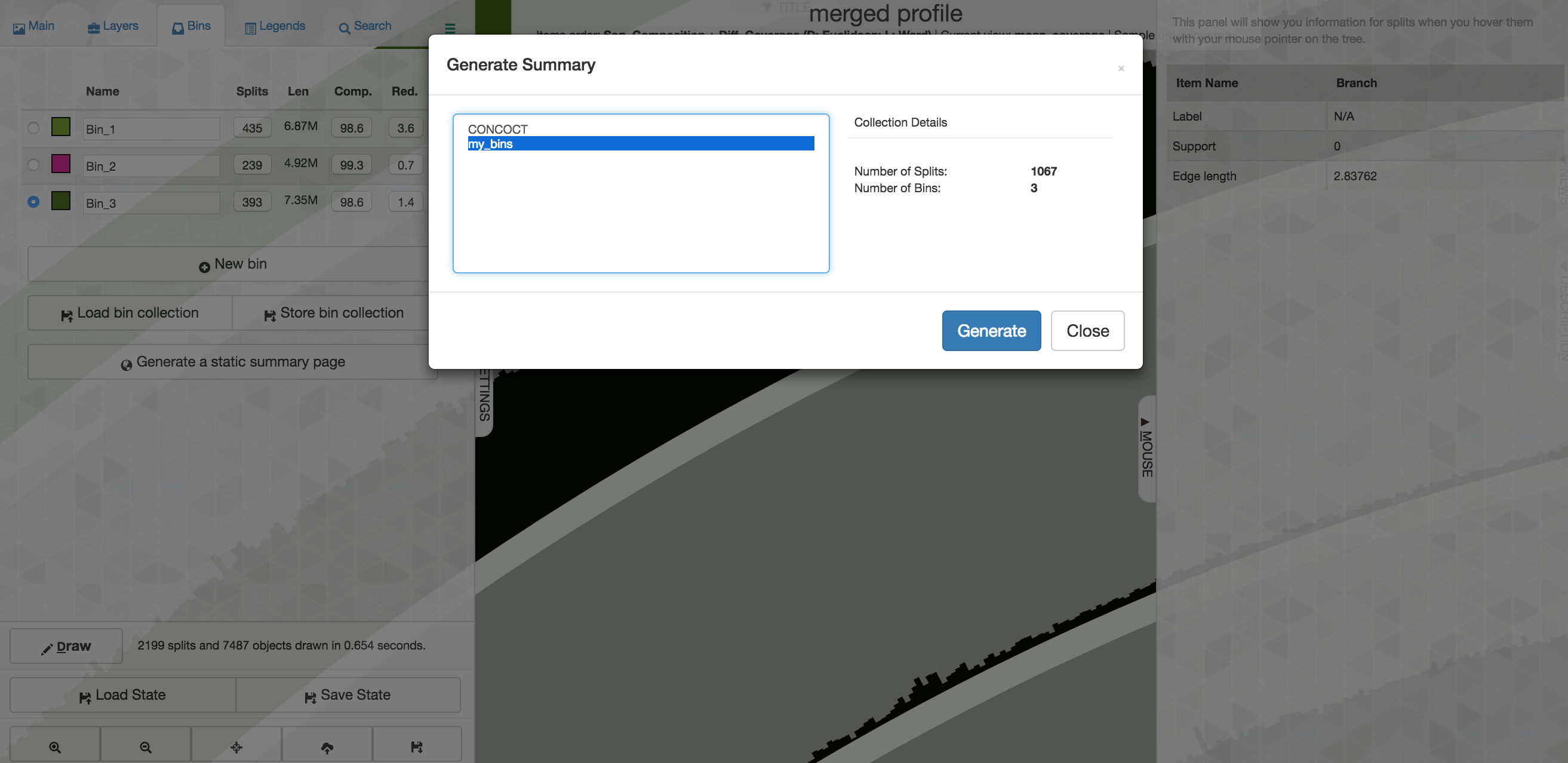
After a few seconds it will finish, and you can click the link to explore an html document summarizing things. When you’re done you can close the browser window and go back to your terminal controlling the cloud instance.

Since we’re done with the interactive mode for now, we can press control + c to cancel the operation in the terminal. Our summary of our bins created a new directory within our merged_profile directory. Within there are more directories of information, including our binned contigs in fasta format. For instance here is where Bin_2’s fasta file (“Bin_2-contigs.fa”) is located:

ls merged_profile/SUMMARY_my_bins/bin_by_bin/Bin_2/

So what now?

There are lots of fun things to do with newly recovered genomes, but unfortunately everything is pretty much beyond what more we can cover here. And as usual, what you want to do next largely depends on what you’re doing all this for anyway. But some ideas could involve things like phylogenomics to robustly place your new genomes within references, looking at distributions of them by recruiting metagenomic reads from other samples and environments, and/or comparative genomics/pangenomics. As mentioned above, anvi’o tutorials, like this one for phylogenomics or this one for pangenomics, are a great place to start 🙂