Things covered here:

• RStudio value and layout
• How to check and set our working directory
• Basic calculations and setting variables
• What indexing is and how to do it
• Reading in and writing out data

Important note!

Maybe the most important thing to keep in mind here is that this is all about exposure, not memorization or mastering anything. Don’t worry about the details. At first we just need to starting building a mental framework of the foundational rules and concepts. That equips us to figure out the things we need to, when we need to do them 🙂

This module is designed for those that are either completely new to R, or have some experience but maybe don’t feel as solid about some of the fundamentals as they’d like. It will run through the very basics such as setting up your working environment, assigning variables, “indexing” (subsetting data), reading in and writing out data. Some relevant terminology is presented here if you find yourself seeing some words that are unfamilar. This page is meant to be a quick-start to get us into and using the R environment.

Part of what makes R so valuable and powerful are all of the open-source packages people have developed for it. We won’t be getting into installing packages here, but there is a separate page here that covers some of the typical avenues for installing packages (and some of the common problems that may arise).

Accessing our R environment

Before we get started, we need an R environment to work in. You can work on your own computer if you’d like, or you can work in a “Binder” that’s been created for this page, see below.

On your computer

It is possible your computer already has R, if you are unsure, you can check by opening a terminal window (a unix-like terminal) and typing R and hitting enter or return. If this launches R rather than giving an error message, you should be good to go (enter q() to exit the R environment). If you do not have R, one way you can install it is with conda as detailed on this page.

With Binder

Binder is an incredible project with incredible people behind hit. I’m still pretty new to it, but the general idea is it makes it easier to setup and share specific working environments in support of open science. What this means for us here is that we can just click this little badge –  – and it’ll open up the proper R environment with all our needed example files in a web-browser ready to rock… how awesome is that?!? So yeah, if you want to work in the binder, click it already!

When that page finishes loading (it may take a couple minutes), you will see a screen like this:

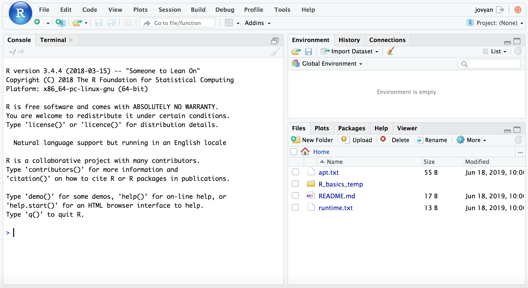
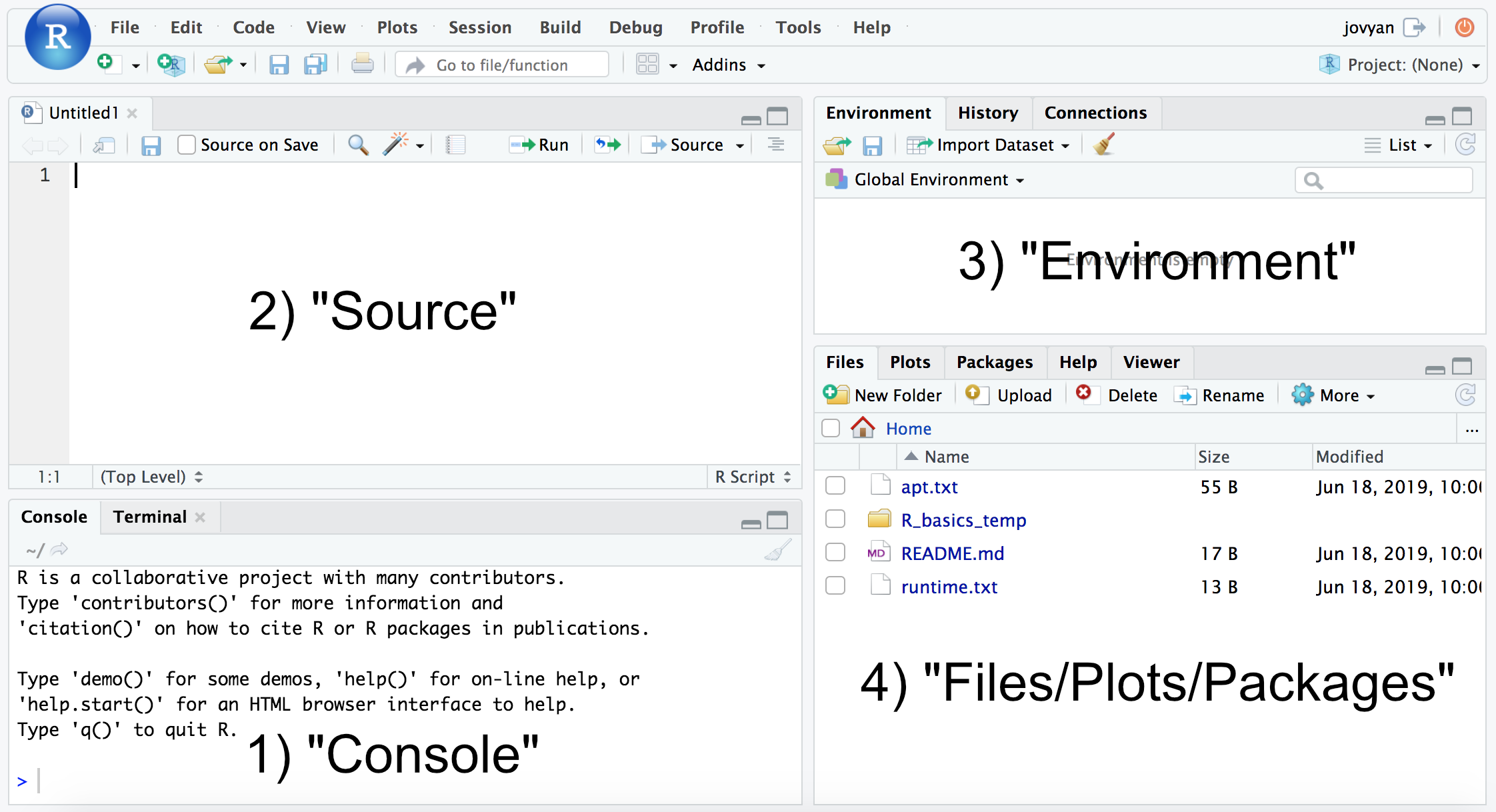
If we then click the icon with the green plus sign at the top-left, and then “R Script”, it will open up our text editor area also, and look something like this (minus the labels added here):

RStudio layout

Whether you are using the binder from above, or installed R and RStudio with conda as described on this page, we now want to be working in RStudio. The typical RStudio has 4 main panes, as numbered above: 1) console; 2) source; 3) Environment; and 4) Files, Plots, Packages, etc. (If you don’t have 4 panes, click the icon with the green plus sign at the top-left, then “R Script”, and it should open the text editor pane.)

1. The “console” is where you can run commands just as though you were working in an R environment at a command line, and it is also where results will print out.
2. The “source” pane acts as a sort-of interactive text editor within which you can write out and save all of your commands, and then call them when you’d like. This is one of the reasons R Studio is great, you’re constantly building up your notes file as you work, without any added effort needed. If you want to run a command written in the source file, while on the line of the command press Cmd + Enter or Ctrl + Enter, or you can highlight a section and do the same to run that section.
3. The “Environment” pane displays all of the variables and data structures you currently have stored.
4. “Files/Plots/Packages/etc.” allows you to navigate your computer in the typical Finder fashion, displays any plots you generate, and serves as your help window.

Here we’re going to be doing our work in the “console” area. To start, let’s see how we can get help on a function. To do this in R, we just place a ? in front of the function name. For example, here is how to see the help info for the function to see what our current working directory is in R:

?getwd

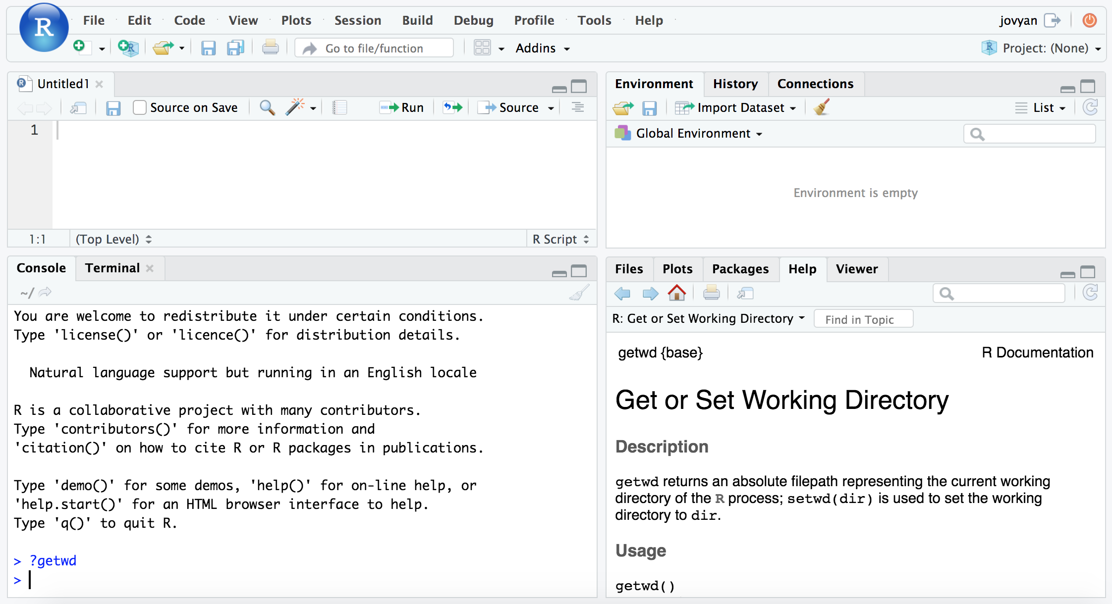
And notice the pane at the bottom right now shows our help info for this function.

Some practice data

If you are not using the binder environment, but want to follow along with this page, copy and paste the following commands into your terminal to get set up with a small, temporary working directory that has the files we’ll be working with. If you’re unfamiliar with working at the command line, and would like to get to know it better, consider running through the Unix crash course here when you can 🙂

cd ~
curl -O https://AstrobioMike.github.io/tutorial_files/R_basics_temp.tar.gz
tar -xvf R_basics_temp.tar.gz
rm R_basics_temp.tar.gz
cd R_basics_temp

Setting up our working environment

Just like when working at the command line, or pointing to files in a graphical user interface program, we need to be aware of “where” we are in our computer when working in R. The getwd() and setwd() help us do this in R. Commands in R typically take this structure, with the command being followed by parentheses (so that’s how we’ll be listing them for the most part here). Inside those parentheses is where the arguments to the command would go if there are any. In the case of getwd() no arguments are needed as it is just going to tell us where we currently are:

getwd()

Note that this is just a zoomed in image of the “console” pane.

However, in the case of setwd(), we then need to tell it where we want to go. Here, we are saying we want to move into the directory holding our example data, and then checking we moved with getwd() again:

setwd("~/R_basics_temp/")
getwd()

NOTE: Here we are providing the absolute path to where we want to go, and it needs to be within quotations. Putting something within quotations in R is what tells it to take the text just as it is, rather than trying to look for a variable that is named with that text. We’ll get into that more later, but just to note now why the quotes are important 🙂

Now that we are in the correct location that should contain the file for our tutorial here, let’s check that it is actually here. At the command line this would be done with the ls command, here in R we do it with the list.files() function.

list.files()

Basic calculations

At its core, R is basically a powerful calculator, so with it we can do baseline arithmetic operations like the following examples. (Don’t forget we are working in the “console” pane as pictured above, these blocks can be copy-and-pasted there if wanted.)

4 + 4
4 / 2
4 * 4
2 ^ 4 

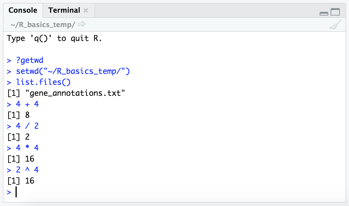
NOTE: The [1] we’re seeing to the left of the output is an “index” number. As we go further we’ll see why these are useful, but for now just know it’s a counter for how many iterms are returned by a command – for each row of printed output it lists the “index” number of the first item of that row, here we only have 1 row of output, so it’s always just showing 1.

Variables in R

Most of the time R acts on things that are stored in variables. In R, things that are stored in variables are referred to as “objects”. Objects can be of different types, and the type of object we are working with (as well as the type of data held within that object) determines what we can and can’t do with that object. This can be super-confusing at first, so don’t worry about it too much right now, but it might be something that is helpful to think about if hitting errors we don’t understand. As you start to spend more time bumping into error messages and googling what’s up, you’ll find that these concepts will more come into focus 👍

In R, we assign values to variables and name them using the assignment operator ( <- ) as shown in the following code block. Here we’re naming the variable “x” (this name could be anything), and giving it a value of 4.

x <- 4

After executing the command, our “environment” pane should now show this variable there.

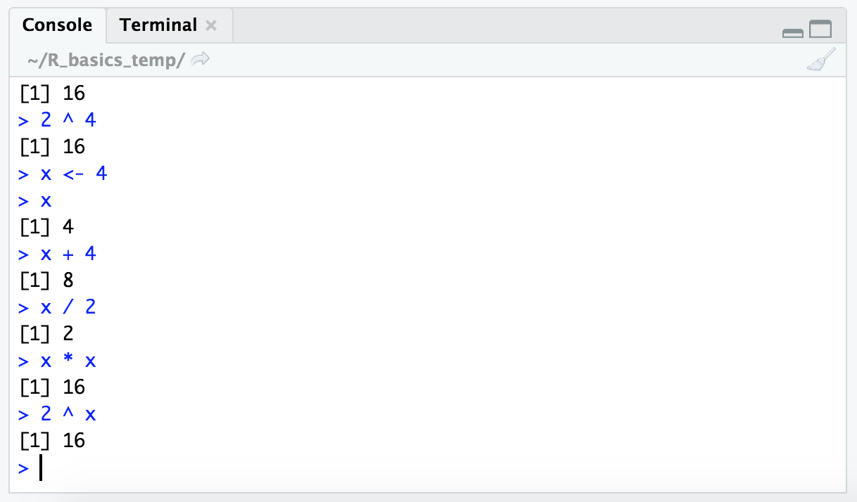
Now that we have the value “4” stored in the variable “x”, we can use the variable name in functions. Here’s some examples doing the same calculations we performed above, but now with our variable.

x
x + 4
x / 2
x * x
2 ^ x

We can also check what type of data is contained within this variable with the class() function:

class(x)

And we find out it is of class “numeric”. Let’s try storing a different type, like a word:

w <- "europa" 
class(w)

NOTE: Here, the class is “character”. Notice again that we need to use quotes when working with characters, like when we set the working directory above. Without the quotes, R will try to find a variable with that name, rather than treating it as plain text. This isn’t the case for numbers, like when we set the variable x to 4 above (this is also why you can’t name a variable starting with a number in R).

class("x")

We can also store multiple items into a single variable. A one-dimensional object holding multiple items is called a vector in R. To put multiple items into one object, we can use the c() function, for “concatenate”. Here we’ll make a vector of numbers:

y <- c(5, 6, 7)
y

Note that this is still of class “numeric” by checking with class(y). It can be helpful to get used to actively being aware of what type of objects we are working with.

Variables can also hold tables. Here we’re going to make another vector with 3 numbers, and then combine it with our previous vector in order to make what’s known as a dataframe (Again, don’t worry about remembering all this terminology right away! This is just about exposure right now.) We’ll do this with the data.frame() function, creating a variable called “our_table”.

z <- c(8, 9, 10)
our_table <- data.frame(y, z)

our_table

class(our_table)

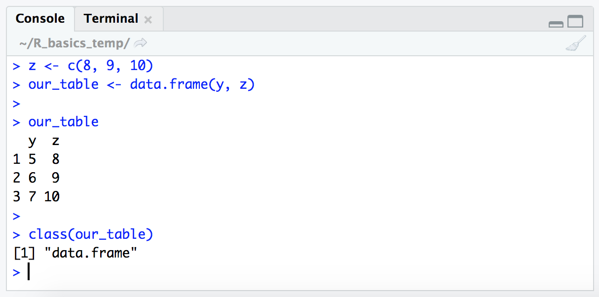
Dataframes are two-dimensional objects of rows and columns. Here we can see that the default behavior of the data.frame() function took our two vectors and put them in a table where each original vector now represents one column. Another similar, but distinct, table structure in R is a “matrix”. You will sometimes find you need to convert a dataframe to a matrix or vice versa depending on what you are trying to do with it. Keep this in mind as one of the things to look at first if you run into an error working with tables.

The wonderful world of indexing

Subsetting tables or vectors in R down to just what we want is sometimes referred to as “indexing”. And it’s a nice concept to be familiar with if working at all in R. Here we’ll look at a couple of the ways we can specify what we would like to subset, and we’ll see these in practice on a larger scale below.

Subsetting by position

Looking back at our vector stored in variable y, it contains 3 values: 5, 6, and 7. These values exist in the object in this order as positions 1, 2, and 3 of the variable y. One way we can subset specific values involves using this position information – this position information for each value is known as that value’s “index”. If we specify the vector name, and then put in brackets [ ] the position(s) we are interested in, R will return the value(s) (things following the # are “comments” that the program ignores).

y # the whole vector
y[1] # the first item
y[2] # second item
y[3] # third item

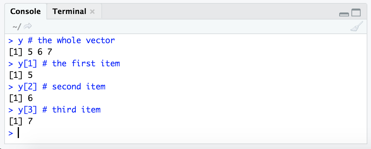
NOTE: It’s good to think about a way to read this syntax that makes sense to us. The variable we are subsetting from comes first, “y” above, then within brackets we are stating what parts of it we want. Here just by index number, so we’re saying something like ‘from object “y”, give us the first item’ (y[1]).

We can also ask for multiple by using the c() function we saw above:

y[c(1,3)] # specifying items 1 and 3

Ok, so that’s how we can subset by saying which positions we want. But in practice we often won’t actually know which positions of a vector hold the values we are interested in – meaning we usually won’t know the “index” number needed to pull out a specific value. This is where another type of indexing comes into play.

Subsetting by conditional statements

Another way to subset via indexing in R makes use of conditional statements. For example, let’s say we wanted all values of our vector y that were greater than or equal to 6. We can subset those values by putting y >= 6 within our subsetting brackets like so:

y # the whole vector
y[y >= 6] # returns just the last two values

The way I read the expression y[y >= 6] in my head is: “Give me all the values of y where y is greater than or equal to 6.”

Conditional statements resolve to TRUE/FALSE

When subsetting by a conditional statement like this, y[y >= 6], R is evaluating what’s in the subsetting brackets to make a logical vector of TRUE and FALSE values, and then only returning the values corresponding to index positions where our TRUE/FALSE vector holds TRUE.

That can sound way more confusing than it is, so let’s look at it real quick, because it’s worth having a bit of an understanding of how this works in order to be able to use it in a broader range of situations 🙂

Here, we’re going to give R a TRUE/FALSE vector in our subsetting brackets:

y
y[c(FALSE, TRUE, TRUE)]

There we typed out a TRUE/FALSE vector, but if we just run y >= 6 by itself, we can see that returns a TRUE/FALSE vector:

y >= 6
# FALSE  TRUE  TRUE

So when we put that conditional statement y >= 6 within our subsetting brackets, R will resolve it to a vector of TRUE/FALSE values and then return only the values for positions where the condition resolves to TRUE:

y 
y[y >= 6]

Now, if we wanted to get the opposite of what our conditional statement yields (so in essence we’d be pulling the values that resolve to FALSE, instead of those that resolve to TRUE), we would add a ! in front of the conditional statement.

We can see this if we just apply it to a vector we type out ourselves:

c(FALSE, TRUE, TRUE)
!c(FALSE, TRUE, TRUE)

This is why putting this in front of our expression like follows will actually give us the opposite result (it will give us the places where the conditional expression we’re providing does not resolve to true):

y

y >= 6
!y >= 6

y[y >= 6]
y[!y >= 6]

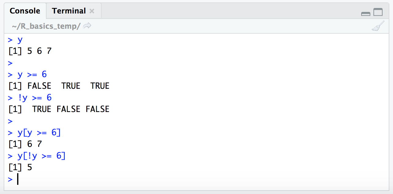
The use of the ! character like this may seem a little unnecessary in the case of strictly numerical conditional expressions like this, but it’s very handy for other types of conditional statements. We’ll see a somewhat more complicated example below where inverting the ! logical vector is the only way to actually get at what we want.

NOTE: Operators such as >, <, and >= as used in the above examples are known as relational operators.

Subsetting tables

So far we’ve been dealing with subsetting just one-dimensional vectors, but similar rules apply to subsetting two-dimensional tables.

As we’ve seen, vectors are one-dimensional objects, so when we want to subset from one we only need to specify details for one coordinate for which item(s) we want. But tables are 2-dimensional objects, so we need to provide instructions for handling two coordinates (one for which rows we’d like and one for which columns).

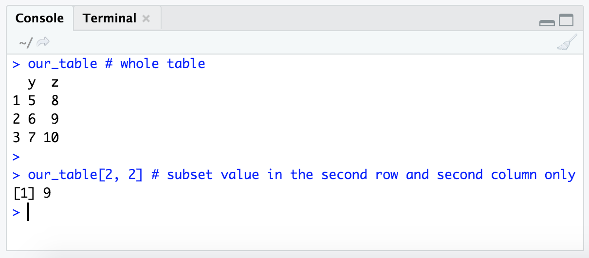
In R, this is still done with the same subsetting brackets ( [ ] ), but now providing two values within them separated by a comma. The first value we enter in the brackets specifies which rows we’d like, and the the second value (separated by a comma) specifies which columns. Using the table we made above, stored in the variable “our_table”, let’s run through some examples of what this looks like:

our_table # whole table

our_table[2, 2] # subset value in the second row and second column only

If we provide nothing for either the row or the column position, but still provide the comma that delineates the two values within our subsetting brackets, we will get all values for that position:

our_table[ , 2] # subset all rows, but only the second column

our_table[3, ] # only row 3, but both columns

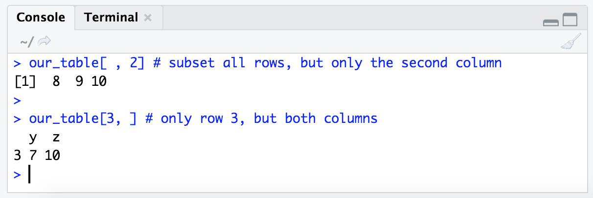
Notice that when subsetting returns only one column, but multiple rows (as in the first example there, our_table[ , 2]), it returns a numeric vector. But when subsetting returns one row, but multiple columns (as in the second example there, our_table[3, ]), it returns a dataframe:

class(our_table[ , 2])

class(our_table[3, ])

This hints at something fundamental about R – that it treats rows and columns differently. This is another detail we don’t need to worry about remembering, but just having seen it once may help troubleshoot faster if we happen to run into it sometime 🙂

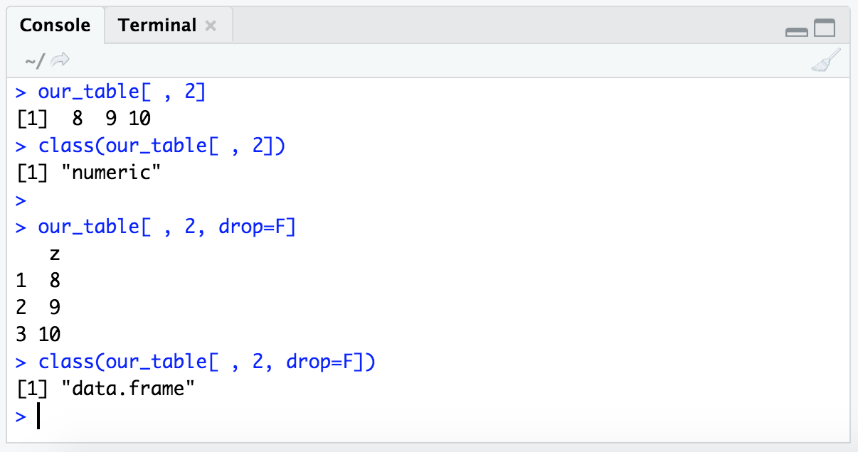
If we want, we can tell R to retain the dataframe structure by adding the optional argument drop=F like so:

our_table[ , 2]
class(our_table[ , 2])

our_table[ , 2, drop=F]
class(our_table[ , 2, drop=F])

Another way we can pull out a specific column from a dataframe as a vector is by the column header/name, in this case we have 2 columns with the names ‘y’ and ‘z’. The function colnames() can tell us this:

colnames(our_table)  

One way we can specify a column we want to pull from a dataframe based on the column name, is to enter the table variable name (here, “our_table”), followed by a $, followed by the column name we want. To get the column named “z” from “our_table”, this looks like this:

our_table$z

We can also do this with the bracket format of subsetting, and therefore combine it with rows by index. Here we are saying we want rows 2 and 3, and specify the column by name instead of its index number:

our_table[c(2,3), "z"]

Notice that we gave the column name within quotes here. This is because we want R to know to just interpret the text and not to look for an object stored in the variable name “z”.

Indexing in R can definitely seem pretty confusing at first, but as mentioned, it is very powerful and a valuable skill while working in R.

Reading in and writing out data

Most of the time when working with R we’re going to want to read in some data, do some stuff to it, and then write out something else to a new file that will then go on to live a wonderous and full life beyond the R environment. Here we’re going to cover the basics of reading in and writing out files.

Checking out the data in the terminal first

Before we try to read data into R, it’s a really good idea to know what we’re expecting. Let’s get some idea of what our example file, “gene_annotations.txt”, looks like in the terminal with some of the tools introduced in the Unix crash course page.

We can work at the terminal in RStudio too, if we click the “Terminal” tab at the top of the “source” pane (which is the bottom left one in our binder environment):

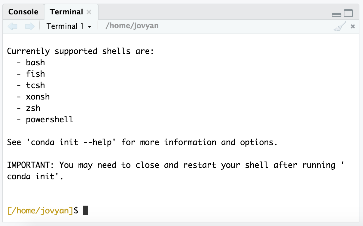
NOTE: If there is a conda error message that pops up before the prompt appears like shown in the image above, we can ignore that.

So in our terminal window, let’s change into the directory holding our example file, and then take a peek at it with less first:

cd ~/R_basics_temp/

less -S gene_annotations.txt # the `-S` prevents lines from wrapping

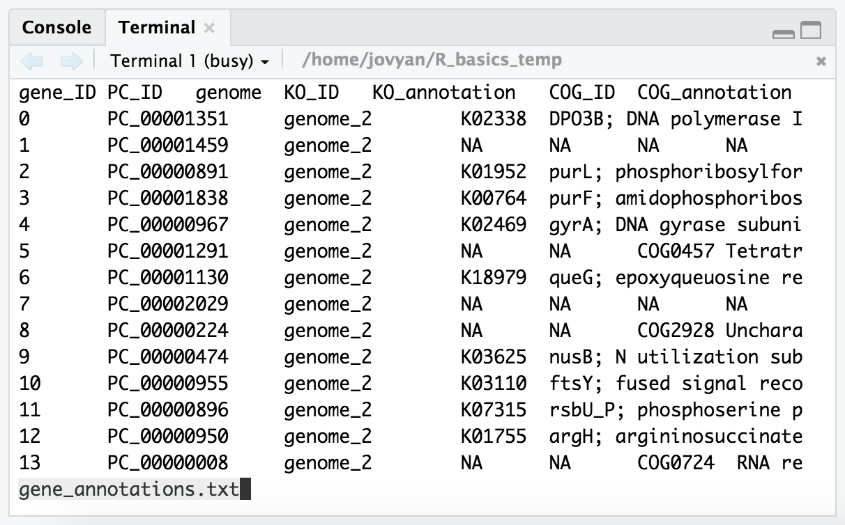
From this we can see that it’s a tab-delimited file, and that it has a header with column names for each column. We can exit less by pressing the q key.

NOTE: It would be more clear that this is a tab-delimited file if I had named it with the “.tsv” extension at the end. I don’t know how I let this slip by at first, I consider that bad practice, but I’ve left it now as an example of what *not to do 🙂

Let’s take a look just at the column names:

head -n 1 gene_annotations.txt

We can also quickly check how many rows we should be expecting:

wc -l gene_annotations.txt

Ok. So now instead of being blind to what the file holds, we know that it’s tab-delimited, it has a header with column names, and it has 8 columns and 84,785 rows (including the header). Awesome. There are some parameters we need to set when we read a file into R, and knowing these things will help us check to make sure we are reading in the file the way we mean to. Now let’s get it into R!

Be sure to switch back to the “Console” tab at the bottom left now, away from the “Terminal” tab, so that our pane looks like this again:

read.table()

One of the most common ways of reading tables into R is to use the read.table() function. To start, let’s try reading our “gene_annotations.txt” table into R with no arguments other than specifying the file name:

gene_annotations_tab <- read.table("gene_annotations.txt")

Yay, our first error! Many error messages may seem a little cryptic at first, but many of them do magically start to make sense over time. The important part in this one is at the end where it says “line 1 did not have 22 elements”. We know from our exploration in the terminal above that our table should have 8 columns. This is a sign there is something up with how R is trying to split each line into columns.

If we take a look at the help menu for this function with ?read.table:

?read.table

The help shows up in our bottom right pane. And scanning through there for anything about specifing the delimiter, we can find the argument “sep”. And it seems that by default the “sep” argument is set to act on all white space, which includes tabs AND blank spaces:

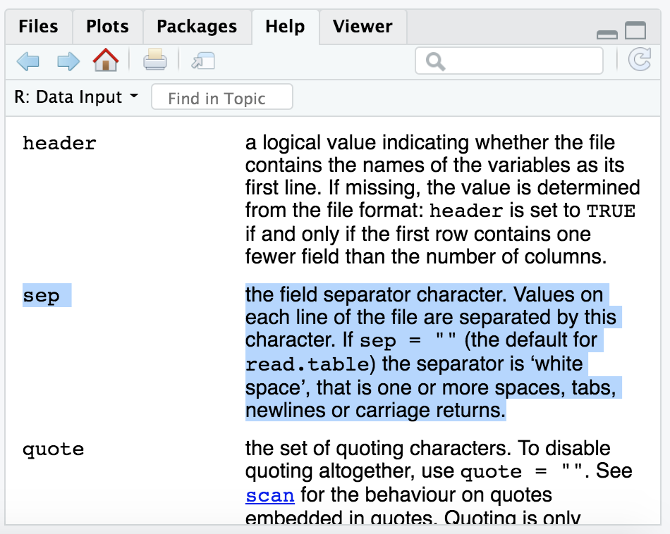
If we remember looking at our “gene_annotations.txt” file in the terminal with less, in addition to it being tab-delimited, there were also spaces within the KO and COG annotation columns.

So read.table() by default is making a new column everywhere there is a space, and then coming back to us and saying “Hey, your first line doesn’t have all the columns it should have based on the rest of your file!” Which is nice of it, because it’s letting us know something is probably wrong 🙂

Let’s try running the command again, but this time stating that the delimiter should only be tabs (tab characters are specified with an backslash followed by a “t” like so: \t.

gene_annotations_tab <- read.table("gene_annotations.txt", sep = "\t")

This works without any errors, let’s take a look at it with the head() function in R:

head(gene_annotations_tab)

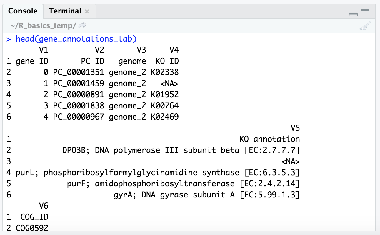
We can ignore that things are wrapping a little funny because it’s wider than the panel can allow, but it put our column names in the first row and added new column names (“V1”, “V2”, etc.), which we definitely don’t want to ignore.

Looking at the help menu for read.table() some more in our bottom right pane, we find there is an argument for “header”, which is by default set to FALSE. So let’s try again but this time we’ll specify that there is a header:

gene_annotations_tab <- read.table("gene_annotations.txt", sep = "\t", header = TRUE)

head(gene_annotations_tab) 

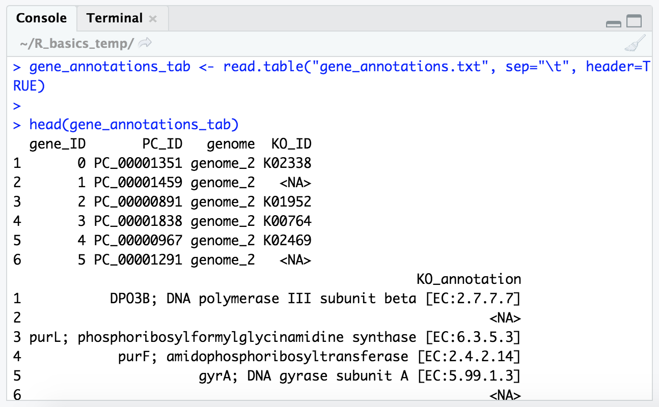
Now we’re gettin’ somewhere. Let’s also check our column names and the size of the table:

colnames(gene_annotations_tab)

dim(gene_annotations_tab)

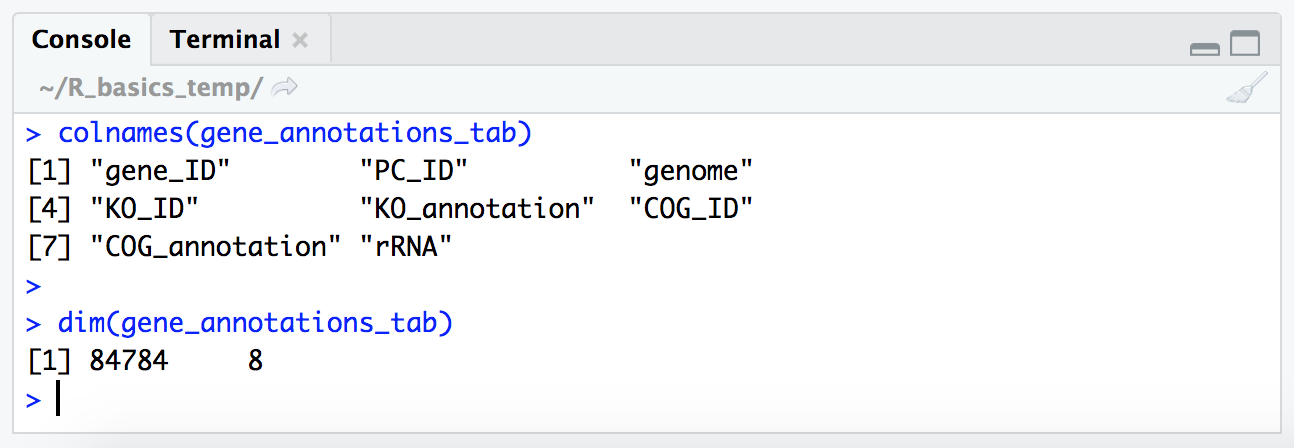
NOTE: Now that our vector of column names is longer than the window (at least in my window when I did this), our index numbers are printed on the left for each row (“[1]”, “[4]”, “[7]”). That is the index (positional number) of each row’s first item.

So our table is 84,784 rows by 8 columns, which is great as that’s what we expect based on what we saw when investigating the file in the terminal.

Now let’s generate a new table so we can practice writing out to a file from R. You may have noticed there are some NAs in our “gene_annotations_tab.txt” table, which are special values to R. These are present in the KEGG and COG annotation and ID columns as “" for those genes which weren't annotated. Here, let's pretend we want to subset our full table down to include only those genes that *were* annotated by KEGG. R's **`is.na()`** function can help us do this. The **`is.na()`** function will return whether or not each item of an object contains an **`NA`**, but in this case we are interested in those that are *not* **`NA`**, meaning we want those that actually contain values (KEGG identifiers in this case). So we need to return the opposite of this using the **`!`** character like we did above with **`y[!y >= 6]`**.

This combines a few concepts, so let’s run the code and then we’ll break it down 🙂

KEGG_only_tab <- gene_annotations_tab[!is.na(gene_annotations_tab$KO_ID), ]

Code Breakdown

• KEGG_only_tab - with this first part we are naming the new variable that will hold our subset table that we are creating
• <- - then we have our assignment operator
• gene_annotations_tab[!is.na(gene_annotations_tab$KO_ID), ] - this is doing our subsetting, just like our smaller example above, but it just looks a little more complicated
  • we first have the starting table gene_annotations_tab
  • then we have our [ ] brackets where we specify how we want to index things
    • in here we have two primary arguments specifying the rows and the columns we want, and they are separated by the , comma
    • !is.na(gene_annotations_tab$KO_ID) is the first, telling us which rows we want
      • saying, “get all the rows where the KO_ID column value is not NA (it would give us all the ones that are NA if we didn’t include the ! upfront)
    • , is the second part, where we are providing nothing specifying which columns, which as mentioned above means to take all of them
  • (revisiting the ‘Conditional statements resolve to TRUE/FALSE’ section above might help if this is still confusing)

And if we peek at our new table with head(), we ses all top 6 have KEGG annotations, where as before some where NA:

head(KEGG_only_tab)

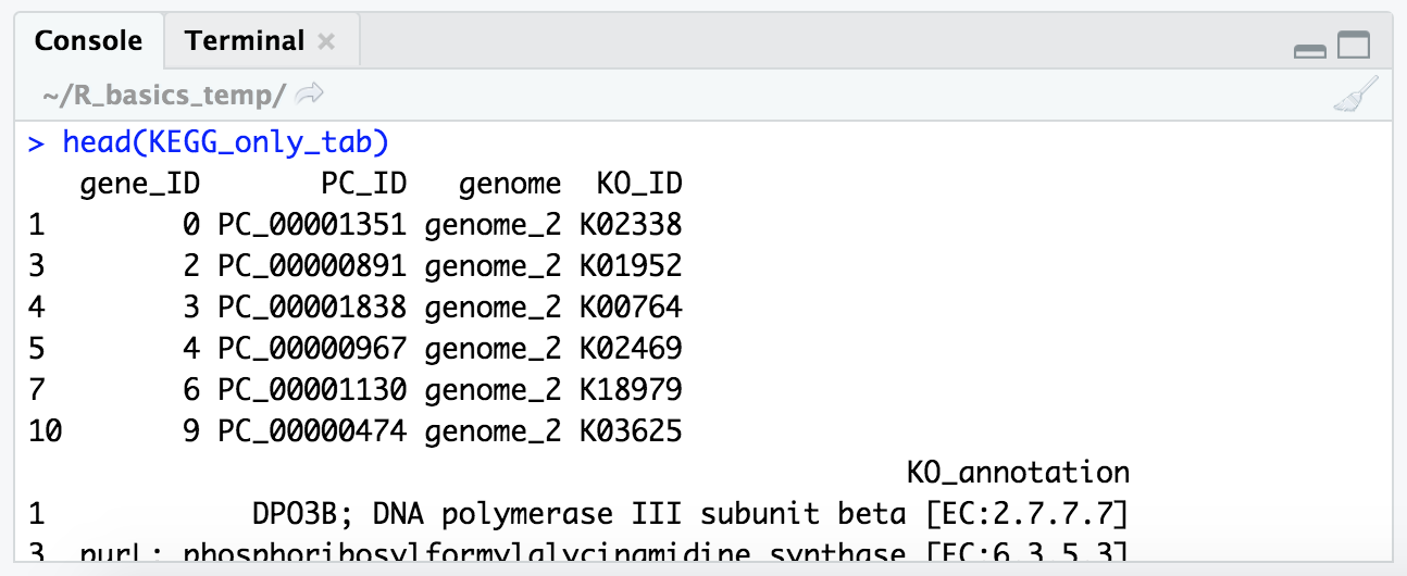
And we can also look at how many genes we dropped that didn’t have a KEGG annotation assigned to them:

dim(gene_annotations_tab) # 84,784 genes
dim(KEGG_only_tab) # 37,319 had KEGG annotations assigned

write.table()

Now, let’s write out our new table of only those genes that were annotated by KEGG to a new tab-delimited file called “KEGG_annotated.tsv” (using a more appropriate extension this time).

We can do this with the write.table() function. If we glance at the help menu for this with ?write.table, we see that the default delimiter (what separates the columns) seems to be a blank space, so we need to be sure to specify that we instead want it to be tab-delimited by providing the argument sep = "\t". We also don’t want to keep the row names R added, so we need to set row.name = FALSE. And by default it will also write out quotation marks around character strings (like our annotation columns) which we also don’t want, so we can set quote = FALSE. How would we know all these things at first? We wouldn’t, ha. Just like above when we were reading in the file, we can write it out and check if things look how we want, and then look up how to get what we want (this is typical to have to do for me even though I use R pretty regularly). So let’s add in these additional arguments to make the file to our liking.

write.table(KEGG_only_tab, "KEGG_annotated.tsv", sep = "\t", row.names = FALSE, quote = FALSE)
list.files() # checking it is there now

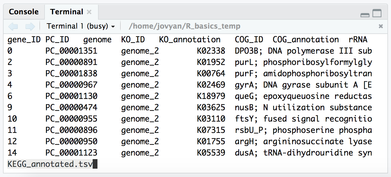
And as mentioned, it’s good practice to peek at the output in the terminal when we are configuring the options to write something out to make sure it’s doing what we think it’s doing. So we can switch back to the “Terminal” tab in the bottom left pane, and check our new file with less:

less -S KEGG_annotated.tsv

BONUS - filtering and piping with the tidyverse

The tidyverse is a collection of R packages for data science. It groups together many incredible useful packages into just one package for us to install and load. There is lots to learn about the tidyverse, but here we are just going to look at two things: how we can “pipe” commands together, and how we can filter or subset tables in a more intuitive fashion that we saw above.

If you are using the binder from above, or a conda-created environment made following the managing R and RStudio with conda page, you will already have the tidyverse package available and can just load it in R by running this:

library(tidyverse)

If you don’t have it available, consider creating doing the conda installation as detailed here, or you will likely be able to install it with the one-line command on this page.

Now that we have that loaded, we’re going to look at doing some filtering the tidyverse way.

We’ll be using the iris dataset, which we have loaded and get get some info on like so:

dim(iris)
# [1] 150   5

head(iris)
#   Sepal.Length Sepal.Width Petal.Length Petal.Width Species
# 1          5.1         3.5          1.4         0.2  setosa
# 2          4.9         3.0          1.4         0.2  setosa
# 3          4.7         3.2          1.3         0.2  setosa
# 4          4.6         3.1          1.5         0.2  setosa
# 5          5.0         3.6          1.4         0.2  setosa
# 6          5.4         3.9          1.7         0.4  setosa

This is a dataset of informatoin about flowers that has 150 rows.

Let’s say we wanted to subset down to only include rows where the Sepal.Length was fewer than 4.5 (not sure what units these are, probably mm ¯\_(ツ)_/¯). The way we could do this with base R would look something like this:

iris[iris["Sepal.Length"] < 4.5, ]
#    Sepal.Length Sepal.Width Petal.Length Petal.Width Species
# 9           4.4         2.9          1.4         0.2  setosa
# 14          4.3         3.0          1.1         0.1  setosa
# 39          4.4         3.0          1.3         0.2  setosa
# 43          4.4         3.2          1.3         0.2  setosa

Where we are givig our subsetting brackets, then building a true/false vector of what we want based on the expression in front of the comma, iris["Sepal.Length"] < 4.5, saying which rows we want to keep (those that yield true from that expression), and implcitly saying we all columns by leaving the argument after the comma blank.

Which is fine, it gets the job done. But it’s kind of annoying to read and annoying to type, and it’s the simplest case of how many things we might want to be filtering on.

Here is the tidyverse way:

iris %>% filter(Sepal.Length < 4.5)
#   Sepal.Length Sepal.Width Petal.Length Petal.Width Species
# 1          4.4         2.9          1.4         0.2  setosa
# 2          4.3         3.0          1.1         0.1  setosa
# 3          4.4         3.0          1.3         0.2  setosa
# 4          4.4         3.2          1.3         0.2  setosa

We’ve introduced two concepts there: the filter() function that comes packaged with tidyverse; and the “pipe” %>% which allows us to string together objects and commands in an arguably more inuitive fashion.

We also could run this as:

filter(iris, Sepal.Length < 4.5)

And get the samet thing, but as we want to stick more things together, it’s generally more intuitive for most people to start with the initial object first, and then keep “piping” it (with the %>% characters) into more functions (similar to how things work at a unix-like command line).

Now let’s say we want to filter for Sepal.Lengh being greater than 6, Petal.Length being greater than or equal to 4.8, and only get those that are of the species versicolor:

iris %>% filter(Sepal.Length > 6, Petal.Length >= 4.8, Species == "versicolor")
#   Sepal.Length Sepal.Width Petal.Length Petal.Width    Species
# 1          6.9         3.1          4.9         1.5 versicolor
# 2          6.3         2.5          4.9         1.5 versicolor
# 3          6.8         2.8          4.8         1.4 versicolor
# 4          6.7         3.0          5.0         1.7 versicolor

That above would be start to get pretty ugly to write out in a base R fashion.

Say we also wanted to then just take the Sepal.Length and Petal.Length columns, we could pipe the end of that into the select() function, which let’s us filter columns, like so:

iris %>% filter(Sepal.Length > 6, Petal.Length >= 4.8, Species == "versicolor") %>% 
    select(Sepal.Length, Petal.Length)
#   Sepal.Length Petal.Length
# 1          6.9          4.9
# 2          6.3          4.9
# 3          6.8          4.8
# 4          6.7          5.0

Note that we can return after the %>% symbol in R, to keep lines shorter and commands easier to read.

Or say we just wanted to know how many there were after our length and species filtering:

iris %>% filter(Sepal.Length > 6, Petal.Length >= 4.8, Species == "versicolor") %>% nrow()
# [1] 4

Or if we wanted to pull just the Petal.Length column out as a vector, to then maybe summarize it, we could use the pull() function (which pulls out the wanted column and converts it to a vector), and then pipe that into the summary() function:

iris %>% filter(Sepal.Length > 6, Petal.Length >= 4.8, Species == "versicolor") %>% 
    pull(Sepal.Length) %>% summary()
  #  Min. 1st Qu.  Median    Mean 3rd Qu.    Max. 
  # 6.300   6.600   6.750   6.675   6.825   6.900

Or if we wanted to save that as a new object, we can still put the new object name and assignment opoerator in front of the whole thing. Like here is doing the filtering above, then storing it in a new object called:

filtered_sepal_length <- iris %>% filter(Sepal.Length > 6, Petal.Length >= 4.8, Species == "versicolor") %>% 
    pull(Sepal.Length)

filtered_sepal_length
# [1] 6.9 6.3 6.8 6.7

The wonderful %>% pipe comes from the magrittr package), and the filtering functions covered above come from the dplyr package (both components included with tidyverse). The above are probably the most commonly used, but there are more awesome functions that come from dplyr, which you can learn more about at its page here if wanted 🙂

Congrats on getting through the basics of R!

R was not immediately intuitive to me (though the tidyverse helps a lot with that!), but it is extremely powerful, many statistical tools are developed to work within it, and it is great for figure generation in addition to just exploring our data. So it’s likely worth the time getting to know R a bit if data science a part of your work 🙂