De novo genome assembly
de novo genome assembly
genomics
Here we’re going to run through some of the typical steps for taking a newly sequenced isolate genome from raw fastq files through to an assembled, curated genome you can then begin to explore. It’s assumed you’re already somewhat familiar with working at the command line, if you’re not yet, you should probably run through the Unix crash course first 🙂
And before we get started here, a public service announcement:
ATTENTION!
This is not an authoritative, exhaustive, or standard workflow for working with a newly sequenced genome. No such thing exists! All genomes, datasets, and goals are different, and new tools are constantly being developed. The point of this page is just to give examples of some of the things you can do, for people who may be completely new to the arena and would benefit from walking through some of these things just for the exposure. Don't let anything here, or anywhere, constrain your science to doing only what others have done!Now that that’s out of the way, let’s get to it!
Tools used here
Throughout this process we’ll be using a variety of tools that I’ve listed below, along with the particular versions I used while putting this together. If you plan to follow along, you’ll need to install these and have them working on your system. The links below go to their respective developer pages where you can usually find great help for installation, but you can also use the wonderful package manager conda to install things.
To get conda up and running (which is very quick), you can follow the instructions to install miniconda (a light-weight version) for your appropriate system starting from here, and then the conda installations below will do the trick.
• FastQC v0.11.5
• Trimmomatic v0.36
• SPAdes v3.11.1
• MegaHit v1.1.1
• QUAST v5.0.2
• bowtie2 v2.2.5
• anvi’o v5.5.0
• centrifuge v1.7.0
Conda installations
This will create an environment for this tutorial and install all these programs at the versions I used when putting this together. At the end there is an example of how to remove this environment, as you will likely want to install the latest versions of these for regular use 🙂
A note on conda
This was initially put together with everything in one conda environment to try to keep things simpler if we weren’t familiar with conda yet. Sometimes that can be a problem if some of the programs have conflicting requirements, or it might also be really slow to install. If having trouble with the below installation, consider running through the conda intro page first, and then break the following up into separate environments and run through this page – just be sure to activate the appropriate environment before a command, and deactivate it after before switching to the next (this will make sense after going through the conda page if it sounds like confusing nonsense right now 🙂). It’d be good practice with conda too, which is super-helpful to become familiar with.
Mamba is generally a much faster reimplementation of the conda infrastructure. So I recommend trying that, particularly if trying large environment builds like this one.
conda install -c conda-forge mamba --yes

mamba create -n de_novo_example -c bioconda -c conda-forge fastqc=0.11.5 \
             trimmomatic=0.36 spades=3.11.1 megahit=1.1.2 quast=5.0.2 \
             bowtie2=2.2.5 anvio=5.5.0 centrifuge=1.0.4 java-jdk=8.0.112 --yes
   # you may or may not need the java-jdk, but it won't hurt our environment :)
And to activate the environment:
conda activate de_novo_example
Or if that gives an error from that, depending on how our conda is set up, we may need to run source activate de_novo_example.
A note on anvio
Anvi’o is a wonderful analysis and visualization platform that is used at the end of this page to give us a visual view of coverage and taxonomy of pieces of our genome assembly. This page was put together a couple of years ago now, and the awesome anvi’o developers are always hard at work improving things and adding new functionality. This page used anvi’o 5.5.0, but many newer versions have come out since. If using a later version, some of the commands in the last section at the bottom of this page might not work the same way. So don’t worry if that’s the case! If wanting to install the latest vesrsion of anvi’o, see their installation page here.
The data
The practice data we’re going to use here was provided by colleagues at the J. Craig Venter Institute. In working out the details for a rather large-scale project, which in part involves sequencing a bunch of Burkholderia isolates from the ISS and performing de novo genome assemblies, Aubrie O’Rourke and her team put an already sequenced isolate – Burkholderia cepacia (ATCC 25416) – through their pipeline in order to test things out and to have something to benchmark their expectations against. The sequencing was done on Illumina’s Nextseq platform as paired-end 2x150 bps, with about a 350-bp insert size.
If you’d like to follow along with this page rather than just reading through, you can download all the data files and execute the commands as below. I tried subsampling the dataset so that things would be smaller and faster for the purposes of this page, but I couldn’t seem to without the assembly suffering too much. By far the most computationally intensive step here is the error correction step, which ended up being the only one that I ran on a server rather than my personal computer (which is a late 2013 MacBook Pro with 4 CPUs and 8GB of memory). So I’ve provided the raw reads and the error-corrected reads so that step can be skipped if wanted. The download also includes most of the intermediate and all of the end-result files so we can explore any component along the way at will without doing the processing. Uncompressed, the whole things is about 1.4 GB:
cd ~
curl -L https://ndownloader.figshare.com/files/15458522 -o genomics_de_novo_temp.tar.gz
tar -xzvf genomics_de_novo_temp.tar.gz && rm genomics_de_novo_temp.tar.gz
cd genomics_de_novo_temp/
Quality filtering
Assessing the quality of our sequence data and filtering appropriately should pretty much always be the first thing we do with our dataset. A great tool to get an overview of what we’re starting with is FastQC. Here we’ll start with that on the raw reads.
FastQC
FastQC scans the fastq files we give it to generage a broad overview of some summary statistics, and has several screening modules that test for some commonly occurring problems. (But as the developers note, its modules are expecitng random sequence data, and any warning or failure notices the program generates should be interpreted within the context of our experiment.) It produces an html output for each fastq file of reads it is given (they can be gzipped). Let’s make sure we are in the proper working directory, and then it can be run like so:
cd ~/genomics_de_novo_temp/working_dir/

fastqc B_cepacia_raw_R1.fastq.gz B_cepacia_raw_R2.fastq.gz -t 4
The resulting html output files can be opened and explored showing all of the modules FastQC scans. Some are pretty straightforward and some take some time to get used to to interpret. It’s also hard to know what to expect when we are looking at the output for the first time without any real baseline experience of what good vs bad examples look like, but the developers provide some files to demonstrate some circumstances. For instance, here is a good example output, and here is a relatively poor one. We should also look over the helpful links about each module provided here.
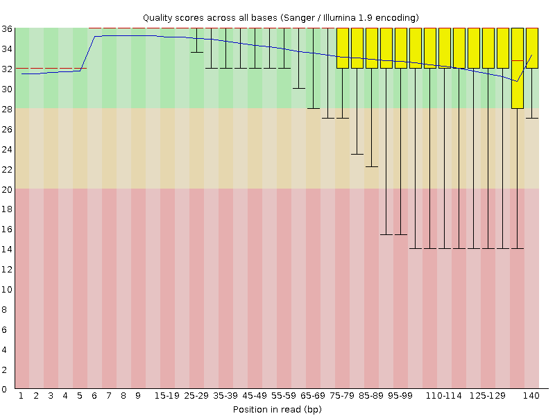
Looking at our output from the forward reads (B_cepacia_raw_R1_fastqc.html), not too much stands out other than the quality scores are pretty mediocre from about 1/3 of the way through the read on:

Here the read length is stretched across the x-axis, the blue line is the mean quality score of all reads at the corresponding positions, red line is the median, and the yellow boxplots represent the interquartile range, and the whiskers the 10th and 90th percentiles. The reverse reads look very similar, we can open that html file (R2) as well if we’d like. Sometimes this will reveal there are still adapters from the sequencing run mixed in, which would wreak havoc on assembly efforts downstream. Getting this type of information from FastQC helps us determine what parameters we want to set for our quality filtering/read trimming.
Trimmomatic
Trimmomatic is a pretty flexible tool that enables us to trim up our sequences based on several quality thresholds and some other metrics (like minimum length or removing adapters and such). Since the summary from FastQC wasn’t all that terrible other than semi-low quality scores, for a first pass I just ran Trimmomatic with pretty generic, but stringent settings:
trimmomatic PE B_cepacia_raw_R1.fastq.gz B_cepacia_raw_R2.fastq.gz \
            BCep_R1_paired.fastq.gz BCep_R1_unpaired.fastq.gz \
            BCep_R2_paired.fastq.gz BCep_R2_unpaired.fastq.gz \
            LEADING:10 TRAILING:10 SLIDINGWINDOW:5:20 MINLEN:151 \
            -threads 4
The syntax for how to run Trimmomatic can be found in their manual, but our filtering thresholds here start with “LEADING:10”. This says cut the bases off the start of the read if their quality score is below 10, and we have the same set for the end with “TRAILING:10”. Then the sliding window parameters are 5 followed by 20, which means starting at base 1, look at a window of 5 bps and if the average quality score drops before 20, truncate the read at that position and only keep up to that point. The stringent part comes in with the MINLEN:151 at the end. Since the reads are already only 151 bps long, this means if any part of the read is truncated due to those quality metrics set above the entire read will be thrown away.
The output from that shows us that only about 14% of the read pairs (both forward and reverse from the same fragment) passed, leaving us with only ~600,000 read pairs. That sounds low, but since we know what we’re working with here (meaning it’s an isolate of a known genus and not a metagenome or something completely unknown), we can pretty quickly estimate if this could even possibly be enough depth for us to assemble the genome we’re expecting. Assuming those reads were perfect quality and perfectly evenly distributed (which they’re not), that would be (600,000 paired reads) * (302 bps per paired read) = 181.2 Mbps covered. Most Burkholderia are around 8.5 Mbps, meaning we’d have around 20X coverage right now, if all were perfect. This confirms that this is a little low and we should probably adjust our stringency on filtering – I don’t think there are solid rules on this either that always hold true, but in my (albeit limited) experience ~50–100X coverage is more around where we want to be for de novo assembly of a typical prokaryotic genome.
So, I went back and altered how I was filtering a bit. Since the worst part of the reads, quality-wise, is at the end, I decided to chop off the last few bps of each read before beginning to do the filtering steps (the parameters we enter into Trimmomatic are carried out in the order in which they appear – though this is usually not the case with most programs at the command line). The length we want to trim the reads down to counts from the 5’ end of each read, and is set with the CROP:140 parameter in the following. And note that the minimum length is now changed too, otherwise nothing would have made it through.
trimmomatic PE B_cepacia_raw_R1.fastq.gz B_cepacia_raw_R2.fastq.gz \
            BCep_R1_paired.fastq.gz BCep_R1_unpaired.fastq.gz \
            BCep_R2_paired.fastq.gz BCep_R2_unpaired.fastq.gz \
            CROP:140 LEADING:10 TRAILING:10 SLIDINGWINDOW:5:20 \
            MINLEN:140 -threads 4
These settings allowed ~36% of paired reads through (~1.5 million pairs), which by the same quick estimation we did above suggests we could possibly have around 50X coverage. 36% is still a low amount of our total starting data, but of course having less “good data”, is better than having more “bad data” – especially when bad sequence data could severly inhibit our assembly efforts.
I decided to move forward with this here. But keep in mind this process doesn’t need to be linear. While we can’t try everything in the world trying to get the best out of our data, sometimes we can try a lot of things (resources and time permitting, of course). So just like we’re going to run a few different assemblers below with different settings and compare them, we could just as easily test different assemblers with different quality-filtered data going into them.
And just for a peek at the FastQC output after our trimming:
fastqc BCep_R1_paired.fastq.gz BCep_R2_paired.fastq.gz -t 4
Things still don’t look perfect, but they look much cleaner than before – now our interquartile boxes (yellow) are much more snuggly sitting up top telling us our distribution of higher qualities across the end of the reads is much better. And though they weren’t much of a factor here, don’t forget to keep an eye on all the other modules from FastQC with any data we throw into it. They are not designed to be perfect assessments, because different experimental conditions can lead to warnings and such for expected reasons as mentioned above, but they are very useful in that they can point us toward potential problems we might not otherwise see. When something does catch our eye, open up the manual for that module here and what it can mean and what can cause it 🙂
Assembly
Now that we have our reads quality filtered, we’re ready to move on to assembling them. There are lots of assembly programs out there, and once again, there is no one-size-fits-all. The data have a lot to say about which assembler is going to work the “best”, and that’s not really a straightforward criterion to shoot for either. I’ve had really good results with SPAdes for isolate or enrichment cultures when I’m trying to reconstruct just one or a few genomes. But when working with high diversity metagenomic samples, sometimes SPAdes can’t handle it and MEGAHIT is pretty awesome with how well it does with such a small memory footprint – and it’s insanely fast.
Whenever I am working with a new dataset, I typically generate a few assemblies testing different programs with different parameters and then compare the results so I can feel at least somewhat confident that I’m doing the best that can currently be done with the data.
Here we’ll run a couple with SPAdes and a couple with MEGAHIT. I will note that I’ve consistently found that incorporating an error-correction step tends improve assembly results, and the one I happen to use is available through the SPAdes program. So even when I end up using the assembly from another program, I typically run error-correction on the reads with SPAdes first, and then put the output of that into whatever other assembler I’m using. A default SPAdes run with the current version (noted at the top of this page) will run the error-correction step and save the reads from it so we can then use them elsewhere. If we don’t want to do the assembly with SPAdes, but run the error-correction step, we can set the --only-error-correction flag like we do first here.
SPAdes
UPDATE: As of SPAdes v3.14, there is a dedicated
--isolatemode that is designed to deal better with the high coverage that typically comes with isolate sequencing. That wasn’t used in the below examples because it wasn’t out yet, but if assembling an isolate, it is probably a good idea to use or at least try that too 🙂
As mentioned above, I’ve had great results with SPAdes before when working with axenic or enrichment cultures, so I anticipate that to be the case here. And as discussed at the top of the page, the error-correction step here is the most computationally intensive of the whole process here, so I ran that alone on a server as follows (it took about 45 minutes with these settings):
# spades.py -1 BCep_R1_paired.fastq.gz -2 BCep_R2_paired.fastq.gz \
#           -o spades_error_corrected_reads -t 50 -m 500 \
#           --only-error-correction
The output files of this are already in our current working directory so that we can take off from this point if we’d like to skip the time-consuming, error-correction step. The forward and reverse error-corrected read files are BCep_R1_QCd_err_cor.fastq.gz and BCep_R2_QCd_err_cor.fastq.gz.
Let’s first run a SPAdes assembly with default settings on the error-corrected reads. Since we already have error-corrected reads, we will provide the flag --only-assembler to tell it not to run the error-correction step. This took about 5–10 minutes on my laptop with 4 threads:
spades.py -1 BCep_R1_QCd_err_cor.fastq.gz -2 BCep_R2_QCd_err_cor.fastq.gz \
          -o spades_default_assembly -t 4 --only-assembler
Or to copy over the results instead of running (if we downloaded the results directory at the top of the page too):
cp -r ../downloaded_results/assemblies/spades_default_assembly/ spades_default_assembly/
And then after doing some scanning of the documentation, I saw this note suggesting specific assembly settings when using 2x150 paired-end Illumina data. It recommends that if we have ~50X or greater coverage (which we were right around based on our rough calculation above), to try setting the kmer lengths to 21,33,55,77, which is the default if our read lengths are at least 150 bps. Since the trimming of the reads we did above put them just under 150 bps long, we’ll have to set that parameter ourselves if we want that last kmer of 77 to be run. That page also suggests running the assembler in --careful mode, which tries to lower the rate of misassemblies. Last, we’ll also be adding the --only-assembler flag again since we’re providing our error-corrected reads (this took about 15 minutes):
spades.py -1 BCep_R1_QCd_err_cor.fastq.gz -2 BCep_R2_QCd_err_cor.fastq.gz \
          -o spades_kmers_set_careful_assembly -t 4 -k 21,33,55,77 \
          --careful --only-assembler
Or we can copy over those results too instead of running:
cp -r ../downloaded_results/assemblies/spades_kmers_set_careful_assembly/ spades_kmers_set_careful_assembly/
MEGAHIT
Next we’ll run two assemblies with MEGAHIT, both on the SPAdes error-corrected reads: one with default settings; and a second using a different --min-count setting as suggested in the developer tips for assembly found here. I didn’t experiment with any without error-correction here, but of course feel free to! These each took about 10 minutes on my computer when ran as follows (or they can also be copied over also as shown after):
  # default
megahit -1 BCep_R1_QCd_err_cor.fastq.gz -2 BCep_R2_QCd_err_cor.fastq.gz \
        -o megahit_default_assembly -t 4

  # changing --min-count parameter
megahit -1 BCep_R1_QCd_err_cor.fastq.gz -2 BCep_R2_QCd_err_cor.fastq.gz \
        -o megahit_min_count_3_assembly -t 4 --min-count 3
Or copying over results instead of running if wanted:
cp -r ../downloaded_results/assemblies/megahit_default_assembly/ megahit_default_assembly/
cp -r ../downloaded_results/assemblies/megahit_min_count_3_assembly/ megahit_min_count_3_assembly/
Now that we have a handful of assemblies done, let’s see how they compare.
Comparing assemblies
Let’s just get this out there right off the bat, there is no individual metric that exists to determine if we have a good assembly or not, especially if we have no reference, and especially especially if we’re working with a metagenomic assembly. There are some general things we can look at, like N50 or largest contig, or fraction of reads that successfully recruit to our assembly, and more. But for one, these don’t really have any solid context to know if they’re “good” or not unless we’re comparing multiple assemblies of the same data; and two, we can have metagenomic assemblies with “worse” overall summary statistics (like N50 and largest contigs), but that might enable us to recover more high-quality bins (or a specific one we know we are looking for) than an assembly with “better” summary metrics. So we have to keep in mind what our goals are, and know that picking the “best” assembly is not a trivial or straightforward task. Having a reference genome like we do in this case however, can make things a lot easier.
QUAST
QUAST is a really nice tool for comparing multiple assemblies, and for metagenome assemblies there is a comparable MetaQUAST. We can provide QUAST with all of our assemblies, a fasta file of our reference genome, and a .gff (general feature format) file of our reference genome that contains information about its genes. I downloaded the two reference files for our Bulkholderia cepacia ATCC 25416 from NCBI here. And here’s how we can run it:
quast -o quast_B_cep_out -R reference_genome/BCep_ref.fna \
      -G reference_genome/BCep_ref.gff \
      -l "spades_default, spades_kmers_careful, megahit_default, megahit_min_count_3" \
      -t 4 -m 1000 spades_default_assembly/contigs.fasta \
      spades_kmers_set_careful_assembly/contigs.fasta \
      megahit_default_assembly/final.contigs.fa \
      megahit_min_count_3_assembly/final.contigs.fa
We can find more about the syntax and how to run QUAST in its documentation. The output directory contains text files of information, but there is also a useful html summary file called “report.html”, which we can open and look at. Here’s a portion of it:
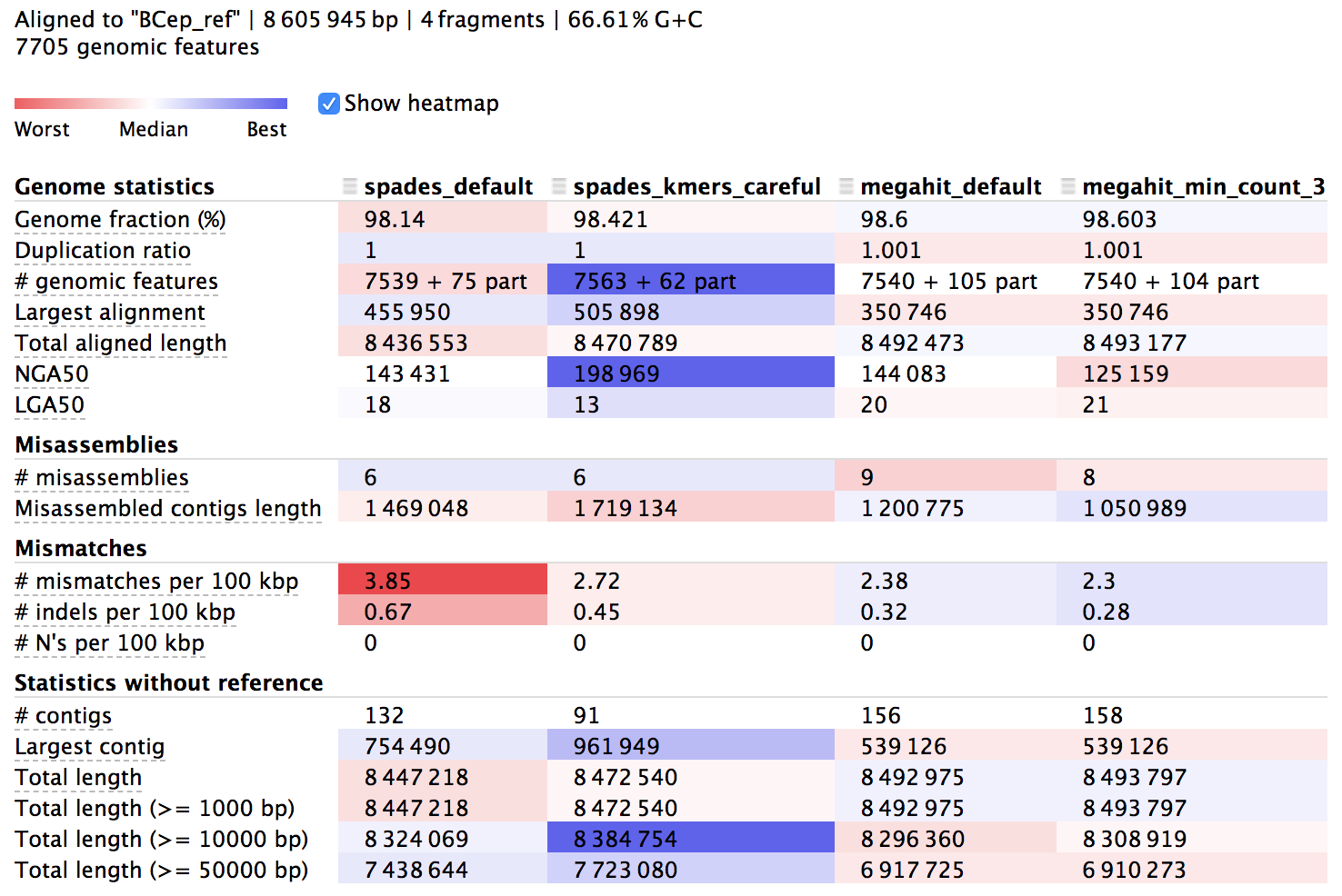
The columns here hold information about each of our 4 assemblies and the rows are different metrics. The majority of the rows starting from the top are in relation to the reference we provided, then the last few starting with “# contigs” are reference-independent. In the interactive html page, we can highlight the row names to get some help on what they mean, and there is more info in the manual of course. The cells are shaded across the assemblies for each row from red to blue, indicating “worst” to “best”, but this is only a loose guide to help our eye, as differences can be negligible or up to interpretation, and some rows are more important than others.
The first thing to notice is that all of them reconstructed over 98% of the reference genome, which I think is pretty stellar, but none of them got 100%. This is to be expected for possibly a few reasons, but most likely it’s just because short Illumina reads alone aren’t able to assemble repetitive regions that extend longer than the paired-read fragment length. We can also see that our assemblies aligned across about 7,550 genes out of the 7,705 that are annotated in the reference genome, and looking at mismatches per 100 kbp we can see we’re down around 2-4 SNVs per 100 kbp – this is no doubt a mixture of sequencing error, assembly error, and actual biological variation – which is close enough to be considered monoclonal in my book (is there a consensus definition for prokaryotes on this?). Moving down to the reference-independent section in the table we can see which assemblies cover the most bps with the fewest contigs. This doesn’t mean everything either, but fewer contigs covering about the same amount of bps does provide more information on synteny, which can be very important.
Read recruitment
Another metric to assess the quality of an assembly is to see how well the reads that went into the assembly recruit back to it. It’s sort of a way of checking to see how much of the data that went in actually ended up getting used. I usually do this for environmental metagenomes, and it has been informative in some cases there, but here – with an isolate genome when the few assemblies tested performed pretty similarly – it turns out that they all pretty much recruited reads just as efficiently (with the default settings of bowtie2 v2.2.5 at least). So I’m leaving the mention of this in here because it can be helpful with some datasets.
As far as selecting which of our assemblies to move forward with, since they all performed reasonably well, mostly for the reason of maximizing insight into synteny as mentioned above, based on the QUAST output I chose to move forward with the SPAdes assembly done with the --careful and specific kmer settings.
What about when we don’t have a reference?
Again, it’s pretty nice here because we have a known reference genome. When that’s not that case, it’s much harder to be confident we are making the best decisions we can. Then I might go further down the path of processing and analysis with multiple assemblies. Some might be better than others for our particular questions, and that might not be decipherable with summary statistics.
For instance, if recovering bins from a metagenomes is the goal, we might want to start that process and see which assembly is better suited for that. As I mentioned above, in at least once case I’ve had better results binning out representative genomes from metagenomic assemblies with seemingly worse overall summary statistics. And if I had just stopped at the assembly summary level, and didn’t run all of them through my binning process as well, I wouldn’t have caught that. Or if our question is more about the functional potential of the whole community, or even looking for specific genes in a metagenome, and not so much about binning things out, then maybe seeing which assembly gives us more open-reading frames or more functional annotations of what we are focusing on could help us decide. The bottom line is it’s difficult, and there is no one answer, but we do the best we can 🙂
Exploring our assembly with anvi’o
A note on anvio
Anvi’o is a wonderful analysis and visualization platform that is used at the end of this page to give us a visual view of coverage and taxonomy of pieces of our genome assembly. This page was put together a couple of years ago now, and the awesome anvi’o developers are always hard at work improving things and adding new functionality. This page used anvi’o 5.5.0, but many newer versions have come out since. If using a later version, some of the commands in the last section at the bottom of this page might not work the same way. So don’t worry if that’s the case! If wanting to install the latest vesrsion of anvi’o, see their installation page here.
Now that we’ve selected the assembly we’re going to move forward with, we can start to take a deeper look at it. And because of how damn glorious it is, anvi’o is a great place to start.
Trying my best to summarize it in one sentence, anvi’o is a very powerful and user-friendly data visualization and exploration platform. It’s powerful mostly because its developers perpetually aim to make it inherently as expansive and flexible as possible, and it’s user-friendly because they actively provide and update loads of well-documented workflows, tutorials, and blog posts. Basically, if you do anything ‘omics-related, I highly recommend getting to know it. There is excellent help on how we can get anvi’o installed here, including the conda way we used above.
As with all things in this vein though, anvi’o isn’t meant to be the “one way” to do things, but rather it is a great platform for integrating many facets of our data. This integration not only facilitates our exploration and can help guide us to where we might want to go deeper, but the underlying infrastructure also contains easily accessible, parsed-down tables and files of lots of information – all waiting for us to investigate specific questions at our whim.
Here we’re going to put our isolate-genome assembly into the anvi’o framework and see just a few of the ways it can help us begin to look at our assembled genome. Many of the major steps we are going to be performing here are laid out in the metagenomic workflow presented here, as much of the processing is the same, and I recommend spending some time reading through that tutorial when you can – whether you have metagenomic data to work with or just isolate or enrichment culture sequencing data. Here, we’re just using anvi’o a bit, and really won’t be digging things, so please be sure to spend some time looking through the anvi’o site to begin exploring its potential.
For us to get our assembly into anvi’o, first we need to generate what it calls a contigs database. This contains the contigs from our assembly and information about them. The following script will organize our contigs in an anvi’o-friendly way, generate some basic stats about them, and use the program Prodigal to identify open-reading frames.
anvi-gen-contigs-database -f spades_kmers_set_careful_assembly/contigs.fasta \
                          -o contigs.db -n B_cepacia_assembly
Now that we have our contigs.db that holds our sequences and some basic information about them, we can start adding more. This is one of the places where the flexibility comes into play, but for now we’ll just move forward with some parts of a general anvi’o workflow, including:
• using the program HMMER with profile hidden Markov models (HMMs) to scan for bacterial single-copy genes and ribosomal RNAs (if new to HMMs, see the bottom of page 7 here for a good explanation of what exactly a “hidden Markov model” is in the realm of sequence data)
• using NCBI COGs to functionally annotate the open-reading frames Prodigal predicted with either BLAST or DIAMOND
• and using a tool called centrifuge for taxonomic classification of the identified open-reading frames
This took ~30 minutes on my laptop, mostly because of needing to download and setup the COG and centrifuge databases for the first time, the following code block doing the mapping took about 10 minutes, and then the anvi-profile step took about 10 minutes. So feel free to skip these next three code blocks and copy over the result files as shown after them to move forward if you’d like 🙂
  # HMM searching for single-copy genes and rRNAs
    # note, if using a newer version of anvi'o, this may need to be
    # changed to "Bacteria_71" instead of "Campbell_et_al"
    # can see those available by running `anvi-run-hmms -h`
anvi-run-hmms -I Campbell_et_al -c contigs.db -T 4
anvi-run-hmms -I Ribosomal_RNAs -c contigs.db -T 4

  # functional annotation with DIAMOND against NCBI's COGs
anvi-setup-ncbi-cogs -T 4 # only needed the first time
anvi-run-ncbi-cogs -c contigs.db --num-threads 4

  # exporting Prodigal-identified open-reading frames from anvi'o
anvi-get-sequences-for-gene-calls -c contigs.db -o gene_calls.fa

  # setting up and running centrifuge for taxonomy
wget ftp://ftp.ccb.jhu.edu/pub/infphilo/centrifuge/data/p_compressed+h+v.tar.gz
tar -xzvf p_compressed+h+v.tar.gz && rm -rf p_compressed+h+v.tar.gz

centrifuge -f -x p_compressed+h+v gene_calls.fa -S centrifuge_hits.tsv -p 4

  # importing the taxonomy results into our anvi'o contigs database
anvi-import-taxonomy-for-genes -c contigs.db -i centrifuge_report.tsv centrifuge_hits.tsv -p centrifuge
The last thing we want to add right now is mapping information from recruiting our reads to the assembly. Here is generating that with bowtie2 and preparing for anvi’o:
  # building bowtie index from our selected assembly fasta file
bowtie2-build spades_kmers_set_careful_assembly/contigs.fasta \
              spades_kmers_set_careful_assembly.btindex
  # mapping our reads
bowtie2 -q -x spades_kmers_set_careful_assembly.btindex \
        -1 BCep_R1_QCd_err_cor.fastq.gz \
        -2 BCep_R2_QCd_err_cor.fastq.gz \
        -p 4 -S spades_kmers_set_careful_assembly.sam
  # converting to a bam file
samtools view -bS spades_kmers_set_careful_assembly.sam > B_cep_assembly.bam
  # sorting and indexing our bam file (can be done with samtools also)
anvi-init-bam B_cep_assembly.bam -o B_cep.bam
We can then integrate this mapping information into anvi’o with the anvi-profile program, which generates another type of database anvi’o calls a “profile database”. There is a lot going on with this step and a lot of things we can play with, discussed here, but for our purposes right now it’s mostly about giving us coverage information for each contig:
  # integrating the read-mapping info into anvi'o
anvi-profile -i B_cep.bam -c contigs.db -M 1000 -T 4 --cluster-contigs -o B_cep_profiled/
If skipping the last 3 code blocks for time, we can copy over the updated contigs.db as follows:
cp ../downloaded_results/anvio_files/contigs.db .
cp -r ../downloaded_results/anvio_files/B_cep_profiled/ B_cep_profiled/
Ok, great, so we’ve just generated and put quite a bit of information about our assembly into our contigs and profile database. And this being anvi’o, it’s now very easy to access specifics of that information when we want it (we can see all of the available programs by typing anvi- and hitting tab twice).
For example, one of the commands we just ran, anvi-run-hmms, searched for ribosomal RNAs and single-copy genes we might be interested in. We can ask anvi’o to give us hits to those HMMs using the anvi-get-sequences-for-hmm-hits (and adding the flag -h will tell us all about how to use the program). Let’s say we want to see what was identified as ribosomal RNA:
anvi-get-sequences-for-hmm-hits -c contigs.db --hmm-sources Ribosomal_RNAs -o rRNAs.fa
This wrote all of the ribosomal RNA hits to a new file called rRNAs.fa, and if we look in that file we see 2 were found, a 16S and a 23S. For our sanity, we can then quickly BLAST them, and in this case be happy because they are both 100% identical to B. cepacia ATCC 25416 (it’s cool when things are actually working, isn’t it?).
We can similarly pull out all of the single-copy genes our bacterial profile HMM searched, translated into their amino acid sequences:
anvi-get-sequences-for-hmm-hits -c contigs.db --hmm-sources Campbell_et_al --get-aa-sequences -o bacterial_SCGs.faa --no-wrap
And sure enough, pulling the “RecA” sequence from that file (e.g., grep -A1 "RecA" bacterial_SCGs.faa) and running a BLASTp on it also gives us 100% identical to our B. cepacia ATCC 25416 reference (well and a lot of other Burkholderia strains since we’re at the amino acid level).
We can also generate some summary statistics on our assembly, including estimated percent completion and redundancy based on the presence/absence of the single-copy marker genes we scanned for above. Here are the two steps needed to summarize our isolate-genome assembly:
  # this is adding all contigs to a group called "DEFAULT"
anvi-script-add-default-collection -p B_cep_profiled/PROFILE.db
  # and here is our summary command
anvi-summarize -c contigs.db -p B_cep_profiled/PROFILE.db -C DEFAULT -o B_cepacia_assembly_summary/
A lot was generated with that, now found in our new directory, “B_cepacia_assembly_summary/”, including an interactive html document we can open and explore. If we glance at the “bins_summary.txt” file we can see some summary statistics of our assembled genome, including the completion/redundancy estimates:
column -ts $'\t' B_cepacia_assembly_summary/bins_summary.txt
# bins        taxon         total_length  num_contigs  N50     GC_content         percent_completion  percent_redundancy
# EVERYTHING  Burkholderia  8472540       91           217699  66.44298758633589  99.28057553956835   1.4388489208633093
Which shows us, in the second column, the majority of taxonomy calls by Centrifuge were actually for the right genus, that’s always nice. Also, based on the Campbell et al. 2013 bacterial single-copy marker genes, our assembly is estimated to be ~99.3% complete with ~1.4% redundancy. But of course this approach doesn’t actually add up to 100% completion and 0% redundancy in all organisms (any?), so for comparison’s sake, I ran the ATCC 25416 reference genome through the same pipeline and got the same results based on this single-copy gene set. Though we are still ~130 Mbps short, as we saw with the QUAST output above.
But great, things look pretty much as they should so far. We can also visually inspect our assembly, and how the reads that went into it recruit to it. In theory, if all the DNA in the assembly came from the same organisms (i.e. it’s a clean assembly), there should be pretty even coverage across the whole thing. So let’s finally take a look with anvi-interactive.
anvi-interactive -c contigs.db -p B_cep_profiled/PROFILE.db --title "B. cepacia assembly"
So there is a lot going on here at first glance, especially if we’re not yet familiar with how anvi’o organizes things. The interactive interface is extraordinarily expansive and I’d suggest reading about it here and here to start digging into it some more when we can, but for our purposes here I’ll just give a quick crash course.
At the center of the figure is a hierarchical clustering of the contigs from our assembly (here clustered based on tetranucleotide frequency and coverage). So each tip (leaf) represents a contig (or a fragment of a contig as each is actually broken down into a max of ~20,000bps, but for right now I’ll just be referring to them as contigs). Then radiating out from the center are layers of information (“Parent”, “Length”, “GC content”, etc.), with each layer displaying information for each contig.
The first thing that jumps out to me here is the outer layer purple, labeled “Taxonomy”. There is actually a color for each contig for whatever taxonomy was assigned to the majority of genes in that particular contig. This solid bar all around tells us that the genes in almost the entire assembly were identified as Burkholderia – minus the one white bar at ~3:00 o’clock which was not classified as anything. The next thing that stands out is how stable the mean coverage is across all contigs, other than mostly just that same area on the right side, where the 2 identified ribosomal RNAs are found. Some areas are expected to have higher coverage like this, particularly ribosomal RNA for our isolate. According to IMG, B. cepacia ATCC 25416 has 7 16S copies and 9 23S copies, which would complicate assembly if they aren’t all identical, and would inflate their coverage compared to the parts of the genome that exist in single copy. Overall this is great and shows the culture really seems to have been axenic.
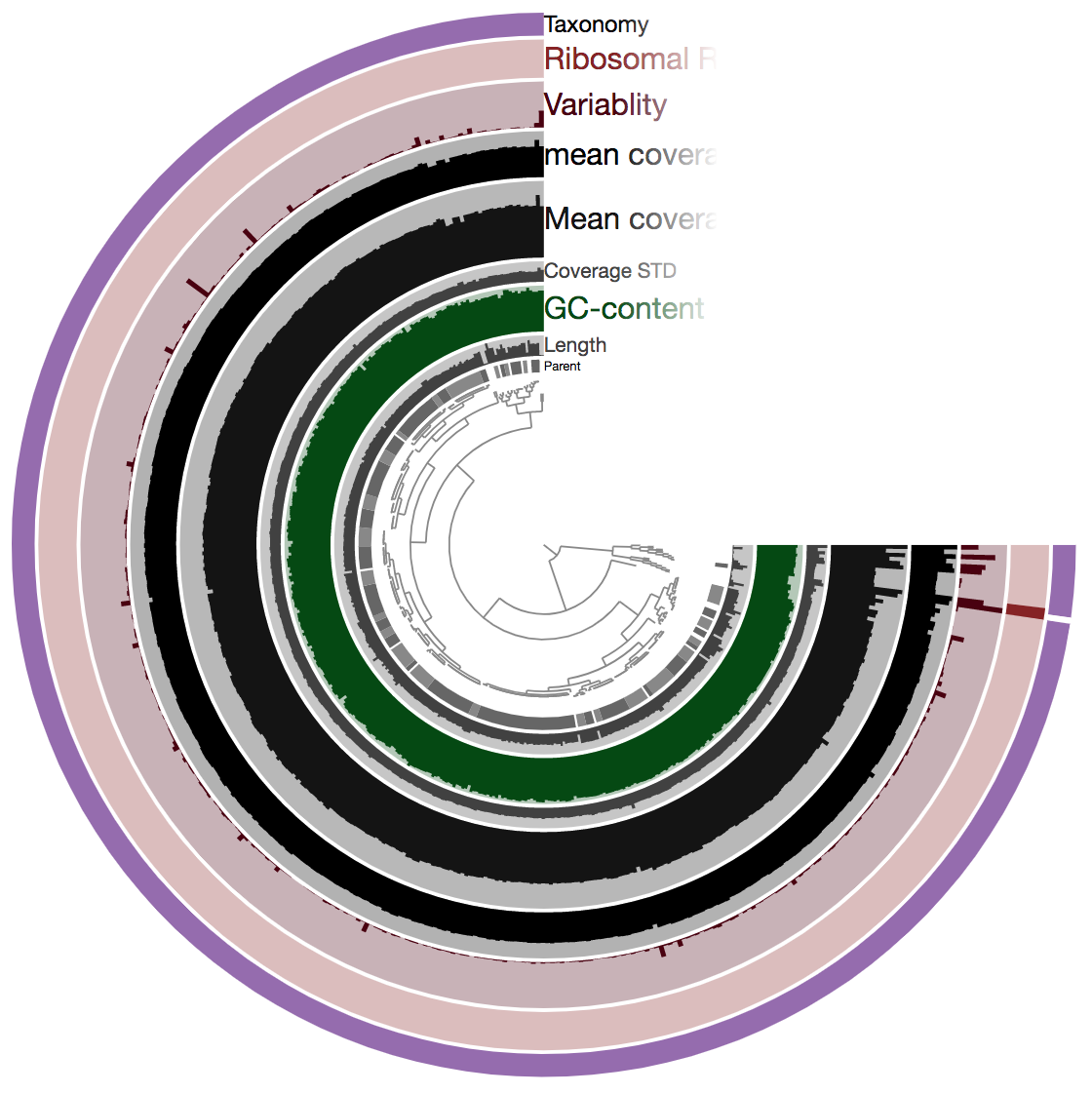
Just for a quick comparison, here is the same type of figure (taxonomy at the inner-part of the circle here), but from an enrichment culture, rather than axenic:
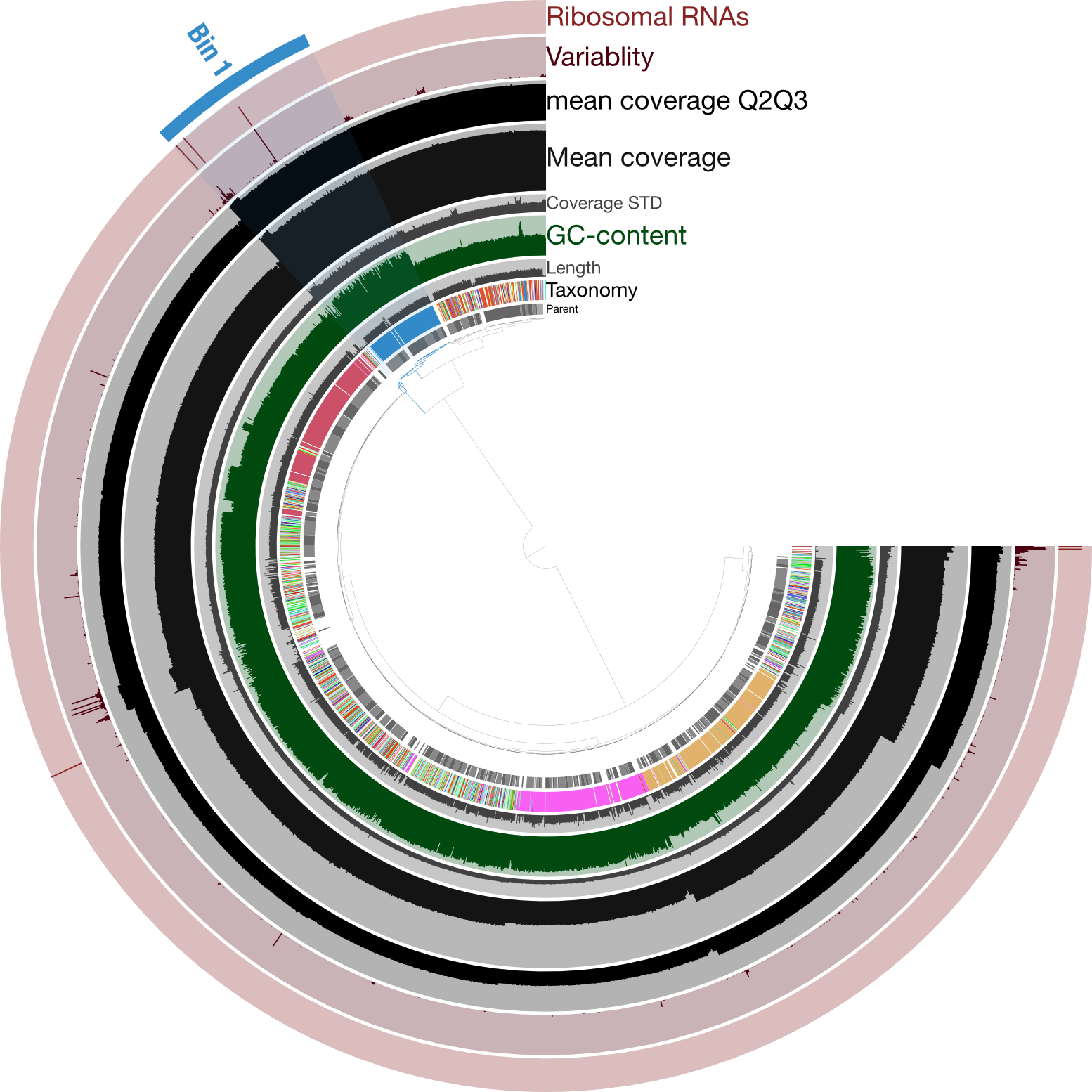
Here the highlighted contigs, labeled “Bin 1”, represent the targeted cultivar from this sequencing run, demonstrating a nice example of how anvi’o can help us manually curate bins we’re trying derive from assemblies.
While we didn’t need much (any) manual curation in this case, it was still a good idea to visually inspect the coverage of our assembly to make sure nothing weird was going on. And if we wanted we could further explore those parts with higher coverage to find out which parts of the genome seem to exist in greater than 1 copy.
If you’d like to remove this conda environment, you can like this:
conda deactivate
conda env remove -n de_novo_example
This was all basically to get a high-quality draft of our isolate genome, that we could feel confident about investigating further. Once you feel comfortable with your assembled genome, you can go a lot of different ways. Going into individual approaches are beyond the scope of this particular page, but here are just a few examples.
A few, of many, possible avenues forward…
Phylogenomics
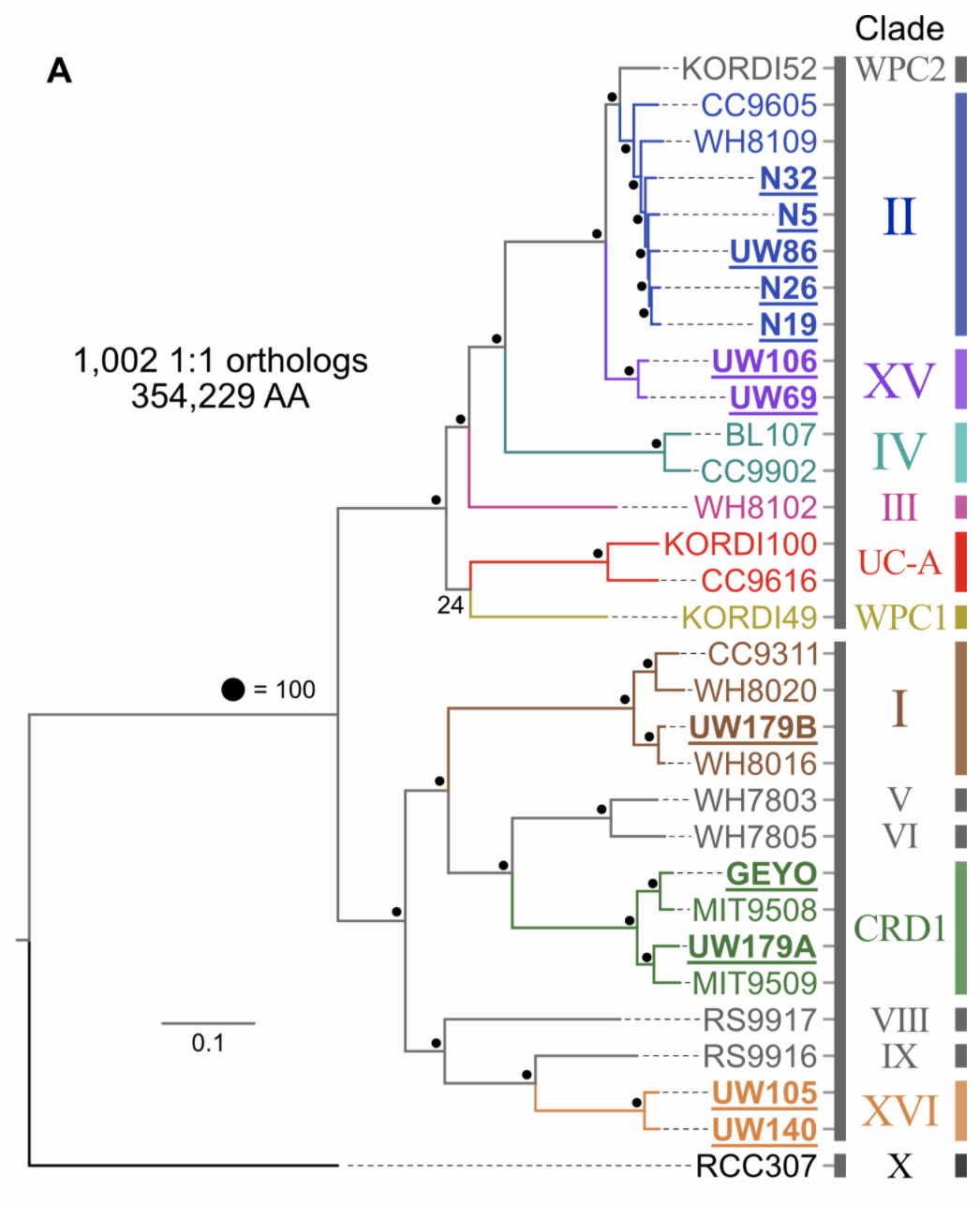
Pull available reference genomes of close relatives and build a phylogenomic tree to get a robust estimate of where your newly acquired isolates fit in evolutionarily with what is already known. Not surprisingly, anvi’o can help you parse this out also. This tree is based on an amino acid alignment of ~1,000 one-to-one orthologs.
Distributions
Pull available metagenomes from other studies and recruit the reads to a reference library containing your isolate (and its close relatives if it has any) to begin assessing the distributions their genomic lineages. This example is done with ocean samples, but the same principle can be applied to any environments.

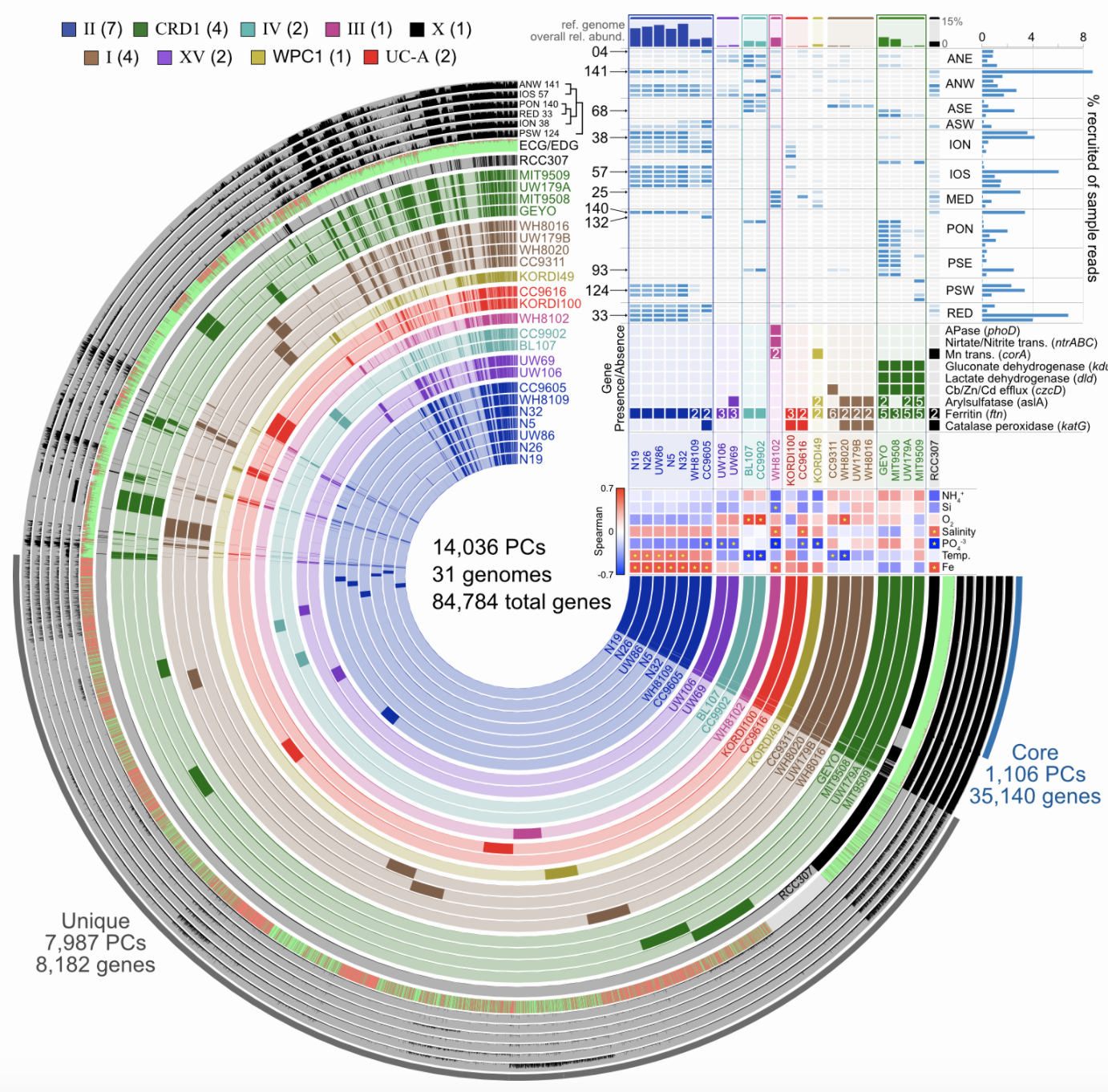
Pangenomics
Start investigating differences in the genetic complement of your new isolate as compared to its known close relatives. And yes, anvi’o can help with that too. This example figure is combining pangenomics (the core of the figure showing the presence or absence of genes within each genome) with metagenomics (distributions of the genomes across samples in the top right corner) to try to associate genomic variability with ecological delineations:
And so much more! Really, just like at the end of the amplicon example workflow, this is where just pure data crunching slows down, and the actual science begins. The above are just some of the ways to get to the point where you can then consider your experimental design and your questions and let them guide where you go next.